1. Quick-start

Authors: Valentin Christiaens and Carlos Alberto Gomez Gonzalez

Suitable for VIP v1.0.0 onwards

Last update: 2022/03/16

Table of contents

• 1.1. Loading ADI data
• 1.2. Model PSF subtraction for ADI
  • 1.2.1. median-ADI
  • 1.2.2. Full-frame PCA

This quick-start tutorial shows:

• how to load Angular Differential Imaging (ADI) datacubes;
• how to use some of the algorithms implemented in VIP to model and subtract the stellar halo in order to produce final post-processed images.

---

Let’s assume VIP and hciplot are properly installed. We import the packages along with other useful libraries:

%matplotlib inline
from matplotlib.pyplot import *
from matplotlib import pyplot as plt
import numpy as np

import vip_hci as vip
from hciplot import plot_frames, plot_cubes

In the following box we import all the routines that will be used in this tutorial. The path to some routines has changed between versions 1.0.3 and 1.1.0, which saw a major revamp of the modular architecture, hence the if statements.

Parts of this notebook will NOT run for VIP versions below 1.0.0.

from packaging import version
vvip = vip.__version__
print("VIP version: ", vvip)
if version.parse(vvip) < version.parse("1.0.0"):
    msg = "Please upgrade your version of VIP"
    msg+= "It should be 1.0.0 or above to run this notebook."
    raise ValueError(msg)
elif version.parse(vvip) <= version.parse("1.0.3"):
    from vip_hci.conf import VLT_NACO
    from vip_hci.medsub import median_sub
    from vip_hci.metrics import normalize_psf
    from vip_hci.pca import pca
else:
    from vip_hci.config import VLT_NACO
    from vip_hci.fm import normalize_psf
    from vip_hci.psfsub import median_sub, pca

# common to all versions:
from vip_hci.fits import open_fits, write_fits, info_fits
from vip_hci.metrics import significance, snr, snrmap
from vip_hci.var import fit_2dgaussian, frame_center

VIP version:  1.2.4

The hciplot package aims to be the “Swiss army” solution for plotting and visualizing multi-dimensional high-contrast imaging datacubes. It replaces the vip_hci.var.pp_subplots function present in older version of VIP. VIP also allows interactive work with DS9 provided that it’s installed on your system along with pyds9. A DS9 session (window) can be started with:

ds9 = vip.Ds9Window()

If the above fails but you have pyds9 installed (vip_ds9 is only a wrapper around pyds9), you may find the following troubleshooting tips useful (e.g. step 4 in particular).

The ds9 methods will allow interaction with the DS9 window. For example, for sending an in-memory array to the DS9 window you can simply use:

ds9.display(2d_or_3d_array)

The above can be used instead of hciplot’s plot_frames and plot_cubes routines (the latter being used in this notebook) for visualization and interaction with your images/datacubes.

1.1. Loading ADI data

In order to demonstrate the capabilities of VIP, you can find in the ‘dataset’ folder of the VIP_extras repository: a toy Angular Differential Imaging (ADI) datacube of images and a point spread function (PSF) associated to the NACO instrument of the Very Large Telescope (VLT). This is an L’-band VLT/NACO dataset of beta Pictoris published in Absil et al. (2013), obtained using the Annular Groove Phase Mask (AGPM) Vortex coronagraph. The sequence has been heavily sub-sampled temporarily to make it smaller. The frames were also cropped to the central 101x101 area. In case you want to plug-in your cube just change the path of the following cells.

Let’s first inspect the fits file:

info_fits('../datasets/naco_betapic_cube_cen.fits')

Filename: ../datasets/naco_betapic_cube_cen.fits
No.    Name      Ver    Type      Cards   Dimensions   Format
  0  PRIMARY       1 PrimaryHDU       7   (101, 101, 61)   float32

The fits file contains an ADI datacube of 61 images 101x101 px across.

The parallactic angle vector for this observation is saved in the naco_betapic_pa.fits file.

Now we load all the data in memory with the open_fits function:

psfname = '../datasets/naco_betapic_psf.fits'
cubename = '../datasets/naco_betapic_cube_cen.fits'
angname = '../datasets/naco_betapic_pa.fits'

cube = open_fits(cubename)
psf = open_fits(psfname)
pa = open_fits(angname)

Fits HDU-0 data successfully loaded. Data shape: (61, 101, 101)
Fits HDU-0 data successfully loaded. Data shape: (39, 39)
Fits HDU-0 data successfully loaded. Data shape: (61,)

open_fits is a wrapper of the astropy fits functionality. The fits file is now a ndarray or numpy array in memory.

If you open the datacube with ds9 (or send it to the DS9 window) and adjust the cuts you will see the beta Pic b planet moving on a circular trajectory, among similarly bright quasi-static speckle. Alternatively, you can use hciplot.plot_cubes:

plot_cubes(cube, vmin=0, vmax=400)

:Dataset   [x,y,time]   (flux)
:Cube_shape     [101, 101, 61]

Note that the parallactic angles are not the final derotation angles to be applied to the images to match north up and east left. The following offsets, taken from Absil et al. (2013), are also added:

derot_off = 104.84 # NACO derotator offset for this observation (Absil et al. 2013)
TN = -0.45         # Position angle of true north for NACO at the epoch of observation (Absil et al. 2013)

angs = pa-derot_off-TN

Let’s measure the Full-Width Half-Maximum (FWHM) by fitting a 2D Gaussian to the core of the unsaturated non-coronagraphic PSF:

%matplotlib inline
DF_fit = fit_2dgaussian(psf, crop=True, cropsize=9, debug=True, full_output=True)

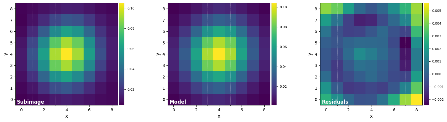
FWHM_y = 4.733218722257407
FWHM_x = 4.473682405059958

centroid y = 19.006680059041216
centroid x = 18.999424475165455
centroid y subim = 4.006680059041214
centroid x subim = 3.9994244751654535

amplitude = 0.10413004853269707
theta = -34.08563676836685

fwhm_naco = np.mean([DF_fit['fwhm_x'],DF_fit['fwhm_y']])
print(fwhm_naco)

4.603450563658683

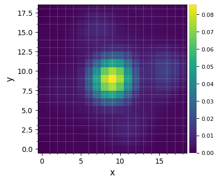
Let’s normalize the flux to one in a 1xFWHM aperture and crop the PSF array:

psfn = normalize_psf(psf, fwhm_naco, size=19, imlib='ndimage-fourier')

Flux in 1xFWHM aperture: 1.228

The normalize_psf function performs internally a fine centering of the PSF (note the input PSF should already be centered within a few pixel accuracy for this fine centering to work). The imlib argument sets the library to be used for sub-px shifts (more details in Tutorial 7).

Let’s visualize the normalized PSF with hciplot.plot_frames. Feel free to adapt the backend argument throughout the notebook: 'matplotlib' allows paper-quality figures with annotations which can be saved (default), while 'bokeh' enables interactive visualization.

plot_frames(psfn, grid=True, size_factor=4)

Let’s finally define the pixel scale for NACO (L’ band), which we get from a dictionary stored in the config subpackage:

pxscale_naco = VLT_NACO['plsc']
print(pxscale_naco, "arcsec/px")

0.02719 arcsec/px

1.2. Model PSF subtraction for ADI

When loading the ADI cube above, we assumed all calibration and preprocessing steps were already performed. In particular, the star is assumed to be already centered in the images. If your data require calibration/preprocessing, feel free to check tutorial 2. Pre-processing for example usage of VIP pre-processing routines on NACO and SPHERE/IFS data.

IMPORTANT - VIP’s convention regarding centering is: - for odd number of pixels along the x and y directions: the star is placed on the central pixel; - for even number of pixels: the star is placed on coordinates (dim/2,dim/2) in 0-based indexing.

All ADI-based algorithms involve image rotation. We therefore first set the preferred method to be used for image rotation. This is controlled with the imlib and interpolation optional arguments (see Tutorial 7. FFT- vs. interpolation-based image operations for more details). Feel free to adapt the following box to test other methods illustrated in Tutorial 7.

imlib = 'vip-fft'
interpolation=None

1.2.1. median-ADI

The most simple approach is to model the PSF with the median of the ADI sequence, subtract it, then derotate and median-combine all residual images (Marois et al. 2006):

fr_adi = median_sub(cube, angs, imlib=imlib, interpolation=interpolation)

――――――――――――――――――――――――――――――――――――――――――――――――――――――――――――――――――――――――――――――――
Starting time: 2022-05-06 10:21:14
――――――――――――――――――――――――――――――――――――――――――――――――――――――――――――――――――――――――――――――――
Median psf reference subtracted
Done derotating and combining
Running time:  0:00:01.445336
――――――――――――――――――――――――――――――――――――――――――――――――――――――――――――――――――――――――――――――――

This can also be done in concentric annuli of annular width asize, considering a parallactic angle threshold delta_rot and the nframes closest images complying with that criterion as model for subtraction to each image of the ADI cube:

fr_adi_an = median_sub(cube, angs, fwhm_naco, asize=fwhm_naco, mode='annular', delta_rot=0.5,
                       radius_int=4, nframes=4, imlib=imlib, interpolation=interpolation)

――――――――――――――――――――――――――――――――――――――――――――――――――――――――――――――――――――――――――――――――
Starting time: 2022-05-06 10:21:16
――――――――――――――――――――――――――――――――――――――――――――――――――――――――――――――――――――――――――――――――
N annuli = 10, FWHM = 4
Processing annuli:
0% [##############################] 100% | ETA: 00:00:00
Total time elapsed: 00:00:00
Optimized median psf reference subtracted
Done derotating and combining
Running time:  0:00:01.806081
――――――――――――――――――――――――――――――――――――――――――――――――――――――――――――――――――――――――――――――――

Note that the parallactic angle threshold corresponding to 0.5 FWHM linear motion could not be met for the innermost annulus, and was therefore automatically relaxed to find nframes eligible frames to be used for the model.

Let’s visualize the final images:

plot_frames((fr_adi, fr_adi_an))

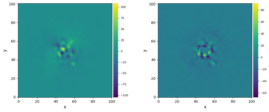
Strong residuals can be seen near the center of the image, with a faint potential point source in the north-east of the final image:

Go to the top

1.2.2. Full-frame PCA

Now let’s try the Principal Component Analysis (PCA) algorithm (Amara & Quanz 2012, Soummer et al. 2012), and set to 5 the number of principal components ncomp considered for model creation.

fr_pca1 = pca(cube, angs, ncomp=5, mask_center_px=None, imlib=imlib, interpolation=interpolation,
              svd_mode='lapack')

――――――――――――――――――――――――――――――――――――――――――――――――――――――――――――――――――――――――――――――――
Starting time: 2022-05-06 10:21:18
――――――――――――――――――――――――――――――――――――――――――――――――――――――――――――――――――――――――――――――――
System total memory = 17.180 GB
System available memory = 1.260 GB
Done vectorizing the frames. Matrix shape: (61, 10201)
Done SVD/PCA with numpy SVD (LAPACK)
Running time:  0:00:01.442372
――――――――――――――――――――――――――――――――――――――――――――――――――――――――――――――――――――――――――――――――
Done de-rotating and combining
Running time:  0:00:02.755106
――――――――――――――――――――――――――――――――――――――――――――――――――――――――――――――――――――――――――――――――

Let’s visualize the final image. This time let’s set the grid option on, to better read coordinates from the image:

plot_frames(fr_pca1, grid=True)

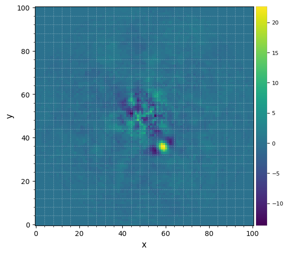
The improvement is clear compared to previous reductions. Very low residuals are seen near the star, and the companion candidate appears as a bright point source surrounded by negative side-lobes.

Now let’s see whether the candidate is significant. For that let’s first set the x,y coordinates of the test point source based on the above image:

xy_b = (58.5,35.5)

Now let’s compute the signal-to-noise ratio at that location, following the definition in Mawet et al. (2014).

snr1 = snr(fr_pca1, source_xy=xy_b, fwhm=fwhm_naco)
print(r"S/N = {:.1f}".format(snr1))

S/N = 8.1

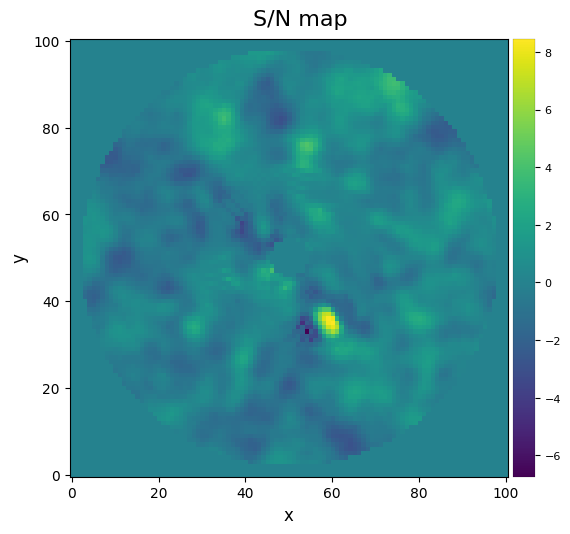
One can also calculate a S/N ratio map over the whole image (this may take a couple of seconds depending on the size of your image):

snrmap1 = snrmap(fr_pca1, fwhm_naco, plot=True)

――――――――――――――――――――――――――――――――――――――――――――――――――――――――――――――――――――――――――――――――
Starting time: 2022-05-06 10:21:21
――――――――――――――――――――――――――――――――――――――――――――――――――――――――――――――――――――――――――――――――

S/N map created using 5 processes
Running time:  0:00:04.991129
――――――――――――――――――――――――――――――――――――――――――――――――――――――――――――――――――――――――――――――――

Remember that S/N ratio is NOT the same as significance (Mawet et al. 2014). Let’s convert the measured S/N ratio (Students statistics) into a Gaussian “sigma” with equivalent false alarm probability. This first involves calculating the radial separation of the candidate:

cy, cx = frame_center(snrmap1)
rad = np.sqrt((cy-xy_b[1])**2+(cx-xy_b[0])**2)

Now let’s use the significance routine in VIP to operate the conversion:

sig = significance(snr1, rad, fwhm_naco, student_to_gauss=True)
print(r"{:.1f} sigma detection".format(sig))

5.4 sigma detection

Congratulations! The detection is significant! You obtained a conspicuous direct image of an exoplanet! Although from this image alone (at a single wavelength) one cannot disentangle a true physically bound companion from a background star, this source has now been extensively studied: it corresponds to the giant planet Beta Pic b (e.g. Lagrange et al. 2009, Absil et al. 2013).

You’re now ready for more advanced tutorials. If you wish to know more about:

• pre-processing functionalities available in VIP (star centering, bad frame trimming, bad pixel correction…) –> go to Tutorial 2;
• more advanced post-processing algorithms –> go to Tutorial 3;
• metrics to evaluate the significance of a detection or the achieved contrast in your image –> go to Tutorial 4;
• how to characterize a directly imaged companion –> go to Tutorial 5;
• how to characterize a circumstellar disk –> go to Tutorial 6;
• the difference between FFT- and interpolation-based image operations (rotation, shifts, scaling) –> go to Tutorial 7;
• the object-oriented implementation of VIP –> go to Tutorial 8.