4. Metrics

Authors: Carlos Alberto Gomez Gonzalez and Valentin Christiaens

Suitable for VIP v1.0.0 onwards

Last update: 2022/05/12

Table of contents

• 4.1. Loading ADI data
• 4.2. Signal-to-noise ratio and significance
  • 4.2.1. S/N map
  • 4.2.2. Significance
  • 4.2.3. STIM map
• 4.3. Automatic detection function
• 4.4. Throughput and contrast curves
  • 4.4.1. Throughput
  • 4.4.2. Contrast curves
• 4.5. Completeness curves and maps
  • 4.5.1. Completeness curves
  • 4.5.2. Completeness maps

This tutorial shows:

• how to compute the S/N ratio of a given companion candidate;
• how to calculate the significance of a detection;
• how to compute S/N ratio maps and STIM maps;
• how to use the automatic point-source detection function;
• how to compute throughput and contrast curves.

---

Let’s first import a couple of external packages needed in this tutorial:

%matplotlib inline
from hciplot import plot_frames, plot_cubes
from matplotlib.pyplot import *
from matplotlib import pyplot as plt
import numpy as np
from packaging import version

In the following box we import all the VIP routines that will be used in this tutorial. The path to some routines has changed between versions 1.0.3 and 1.1.0, which saw a major revamp of the modular architecture, hence the if statements.

import vip_hci as vip
vvip = vip.__version__
print("VIP version: ", vvip)
if version.parse(vvip) < version.parse("1.0.0"):
    msg = "Please upgrade your version of VIP"
    msg+= "It should be 1.0.0 or above to run this notebook."
    raise ValueError(msg)
elif version.parse(vvip) <= version.parse("1.0.3"):
    from vip_hci.conf import VLT_NACO
    from vip_hci.medsub import median_sub
    from vip_hci.metrics import cube_planet_free, normalize_psf, snr, snrmap
    from vip_hci.metrics import compute_stim_map as stim_map
    from vip_hci.metrics import compute_inverse_stim_map as inverse_stim_map
    from vip_hci.pca import pca, pca_annular
else:
    if version.parse(vvip) >= version.parse("1.2.4"):
        from vip_hci.metrics import completeness_curve, completeness_map
    from vip_hci.config import VLT_NACO
    from vip_hci.fm import cube_planet_free, normalize_psf
    from vip_hci.metrics import inverse_stim_map, snr, snrmap, stim_map
    from vip_hci.psfsub import median_sub, pca, pca_annular

# common to all versions:
from vip_hci.fits import open_fits, write_fits, info_fits
from vip_hci.metrics import contrast_curve, detection, significance, snr, snrmap, throughput
from vip_hci.preproc import frame_crop
from vip_hci.var import fit_2dgaussian, frame_center

VIP version:  1.2.4

4.1. Loading ADI data

In the ‘dataset’ folder of the VIP_extras repository you can find a toy ADI (Angular Differential Imaging) cube and a NACO point spread function (PSF) to demonstrate the capabilities of VIP. This is an L’-band VLT/NACO dataset of beta Pictoris published in Absil et al. (2013) obtained using the Annular Groove Phase Mask (AGPM) Vortex coronagraph. The sequence has been heavily sub-sampled temporarily to make it smaller. The frames were also cropped to the central 101x101 area. In case you want to plug-in your cube just change the path of the following cells.

More info on this dataset, and on opening and visualizing fits files with VIP in general, is available in Tutorial 1. Quick start.

Let’s load the data:

psfnaco = '../datasets/naco_betapic_psf.fits'
cubename = '../datasets/naco_betapic_cube_cen.fits'
angname = '../datasets/naco_betapic_pa.fits'

cube = open_fits(cubename)
psf = open_fits(psfnaco)
pa = open_fits(angname)

Fits HDU-0 data successfully loaded. Data shape: (61, 101, 101)
Fits HDU-0 data successfully loaded. Data shape: (39, 39)
Fits HDU-0 data successfully loaded. Data shape: (61,)

derot_off = 104.84 # NACO derotator offset for this observation (Absil et al. 2013)
TN = -0.45         # Position angle of true north for NACO at the epoch of observation (Absil et al. 2013)

angs = pa-derot_off-TN

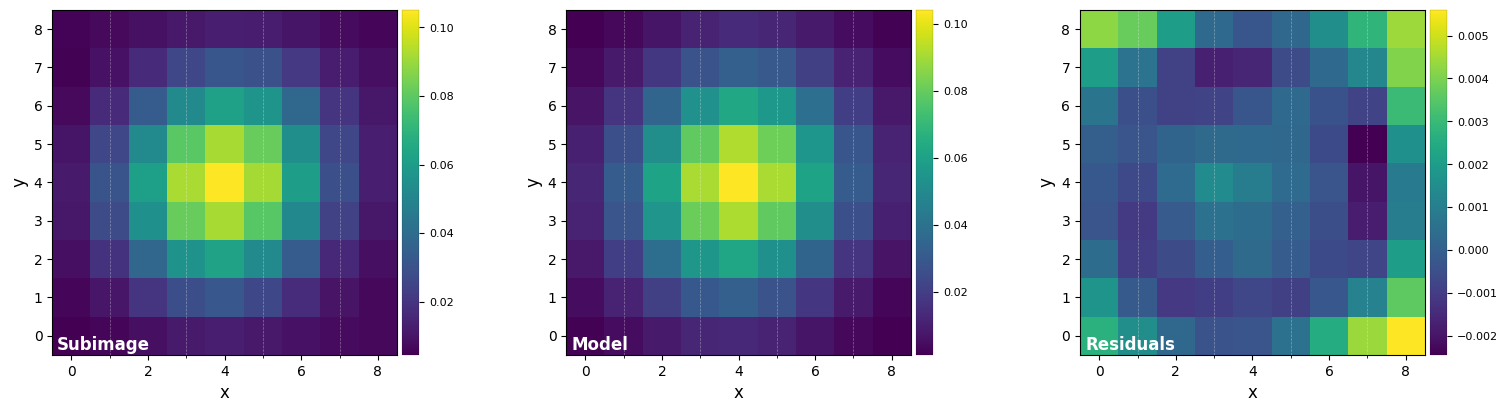
Let’s measure the FWHM by fitting a 2D Gaussian to the core of the unsaturated non-coronagraphic PSF:

%matplotlib inline
DF_fit = fit_2dgaussian(psf, crop=True, cropsize=9, debug=True, full_output=True)

FWHM_y = 4.733218722257407
FWHM_x = 4.473682405059958

centroid y = 19.006680059041216
centroid x = 18.999424475165455
centroid y subim = 4.006680059041214
centroid x subim = 3.9994244751654535

amplitude = 0.10413004853269707
theta = -34.08563676836685

fwhm_naco = np.mean([DF_fit['fwhm_x'],DF_fit['fwhm_y']])
print(fwhm_naco)

4.603450563658683

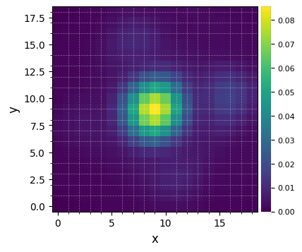
Let’s normalize the flux to one in a 1xFWHM aperture and crop the PSF array:

psfn = normalize_psf(psf, fwhm_naco, size=19, imlib='ndimage-fourier')

Flux in 1xFWHM aperture: 1.228

plot_frames(psfn, grid=True, size_factor=4)

Let’s finally define the pixel scale for NACO (L’ band), which we get from a dictionary stored in the conf subpackage:

pxscale_naco = VLT_NACO['plsc']
print(pxscale_naco, "arcsec/px")

0.02719 arcsec/px

4.2. Signal-to-noise ratio and significance

4.2.1. S/N map

When testing different stellar PSF modeling and subtraction algorithms, one may end up with a point-like source in the final post-processing images. How can its signal-to-noise ratio be assessed?

By default we adopt the definition of S/N given in Mawet el al. (2014), which uses a two samples t-test for the problem of planet detection. Student (t) statistics are relevant for hypothesis testing in presence of a small sample. Since the structure of speckle noise varies radially, this is the case of high contrast imaging of point sources at small angles.

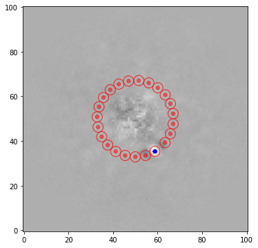
The main idea is to test the flux of a given speckle or planet candidate against the flux measured in resolution elements at the same radial separation from the center:

\[S/N≡ \frac{\overline{x}_1 - \overline{x}_2}{s_2\sqrt{1+\frac{1}{n_2}}},\]

where \(\overline{x}_1\) is the flux of the tested resolution element (blue dot in the figure below), \(\overline{x}_2\) and \(s_2\) are the mean and empirical standard deviation of the fluxes of the background resolution elements (red dots in the figure below) and \(n_2\) the number of such background resolution elements.

Let’s illustrate this process on a PCA post-processed image which contains a companion candidate:

pca_img = pca(cube, angs, ncomp=6, verbose=False, imlib='vip-fft', interpolation=None)
plot_frames(pca_img, backend='bokeh')

Let’s define the coordinates of a test point source in the image:

xy_b = (58.8,35.3)

The snr function in the metrics module can be used to estimate the S/N ratio of the point source:

snr1 = snr(pca_img, source_xy=xy_b, fwhm=fwhm_naco, plot=True)
snr1

7.070108817378683

The S/N is relatively high, however we see that one of the test apertures is overlapping with one of the two negative side lobes (which is the typical signature for a point-source imaged with ADI). The exclude_negative_lobes option can be set to avoid considering apertures right next to the test aperture, which can make a significant difference in terms of S/N ratio in some cases:

snr1 = snr(pca_img, source_xy=xy_b, fwhm=fwhm_naco, plot=True, exclude_negative_lobes=True)
snr1

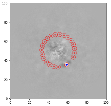
13.77946796804528

One has to be careful with the exclude_negative_lobes option though, as it decreases the number of test apertures, hence increases the small-angle penalty factor.

In the metrics subpackage we have also implemented a function for S/N map generation, by computing the S/N for each pixel of a 2D array. It has a parameter nproc for exploiting multi-core systems which by default is None, meaning that it will use half the number of available CPUs in the system.

snrmap_1 = snrmap(pca_img, fwhm=fwhm_naco, plot=True)

――――――――――――――――――――――――――――――――――――――――――――――――――――――――――――――――――――――――――――――――
Starting time: 2022-05-12 12:28:26
――――――――――――――――――――――――――――――――――――――――――――――――――――――――――――――――――――――――――――――――

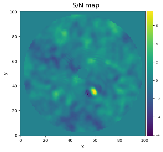
S/N map created using 5 processes
Running time:  0:00:03.314252
――――――――――――――――――――――――――――――――――――――――――――――――――――――――――――――――――――――――――――――――

In case we really need the S/N map of a big frame (which can take quite some time to compute depending on your hardware), a good option is to use the approximated=True option. It uses an approximated S/N definition that yields close results to the one mentioned earlier.

snrmap_f = snrmap(pca_img, fwhm=fwhm_naco, plot=True, approximated=True)

――――――――――――――――――――――――――――――――――――――――――――――――――――――――――――――――――――――――――――――――
Starting time: 2022-05-12 12:28:29
――――――――――――――――――――――――――――――――――――――――――――――――――――――――――――――――――――――――――――――――

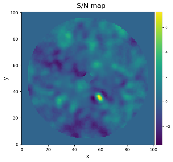
S/N map created using 5 processes
Running time:  0:00:00.425865
――――――――――――――――――――――――――――――――――――――――――――――――――――――――――――――――――――――――――――――――

Question 4.1: In the presence of azimuthally extended disc signals in the field of view, how do you expect the S/N ratio of authentic sources to behave? Would the classical definition above still be reliable, or would it underestimate/overestimate the true S/N ratio of authentic circumstellar signals?

4.2.2. Significance

Due to the common confusion between S/N ratio and significance, we have included a routine to convert (Student) S/N ratio (as defined above) into a Gaussian “sigma” significance, which is the most common metrics used to assess significance in signal detection theory.

The conversion is based on matching the false positive fraction (FPF; e.g. \(3 \times 10^{-7}\) for a \(5\sigma\) detection threshold), or equivalently the confidence level CL = 1-FPF.

As an example, let’s consider a second tentative source (arguably point-like) in our Beta Pic dataset:

xy_test = (55.6, 59.7)
snr2 = vip.metrics.snr(pca_img, source_xy=xy_test, fwhm=fwhm_naco, plot=True, exclude_negative_lobes=True)
print(snr2)

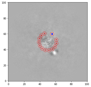
3.1943589456667882

The first point source (as shown in Sec. 4.2.1.) has a very high S/N of ~13.8. The second point-like source has a S/N ~3.2. What is the significance level that each blob is an authentic point source detection (i.e. not a residual speckle emerging randomly as part of the residual intensity distribution)?

The significance routine in the metrics module takes into account both the S/N ratio and the radial separation of the point source (the FWHM is also required to express that radial separation in terms of FWHM), for conversion to significance in terms of Gaussian statistics.

from vip_hci.metrics import significance
from vip_hci.var import frame_center
cy, cx = frame_center(cube[0])
rad1 = np.sqrt((cy-xy_b[1])**2+(cx-xy_b[0])**2)
rad2 = np.sqrt((cy-xy_test[1])**2+(cx-xy_test[0])**2)
sig1 = significance(snr1, rad1, fwhm_naco, student_to_gauss=True)
sig2 = significance(snr2, rad2, fwhm_naco, student_to_gauss=True)
msg = "The point-like signal with S/N={:.1f} at r = {:.1f}px ({:.1f} FWHM radius) corresponds to a {:.1f}-sigma detection (Gaussian statistics)."
print(msg.format(snr1, rad1, rad1/fwhm_naco, sig1))
print(msg.format(snr2, rad2, rad2/fwhm_naco, sig2))

The point-like signal with S/N=13.8 at r = 17.1px (3.7 FWHM radius) corresponds to a 6.9-sigma detection (Gaussian statistics).
The point-like signal with S/N=3.2 at r = 11.2px (2.4 FWHM radius) corresponds to a 2.7-sigma detection (Gaussian statistics).

The first point-like signal appears to be an authentic circumstellar point source (i.e. a physical companion or background object) given that its confidence level is equivalent to that of a \(6.9\sigma\) detection (Gaussian sigma). For the second blob, the confidence level is equivalent to that of a \(2.7\sigma\) detection (Gaussian statistics) - i.e. it is not a significant detection.

Question 4.2: How can one disentangle a physically bound companion (planet, brown dwarf of stellar binary) from a background object?

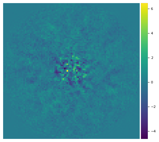
4.2.3. STIM map

In the presence of extended disc signals, an alternative to the S/N map is to use the Standardized Trajectory Intensity Map (STIM; Pairet et al. 2019). A comparison between S/N and STIM maps for disc signals in the system of PDS 70 can be found in Christiaens et al. (2019a).

The STIM map is defined by:

\[{\rm STIM}(x,y) \equiv \frac{\mu_z(x,y)}{\sigma_z(x,y)},\]

where \(\mu_z\) and \(\sigma_z\) are the temporal mean and standard deviation of the derotated residual cube across the temporal dimension, respectively. It is calculated for each pixel (x,y).

Let’s calculate it for our Beta Pictoris L’-band test dataset. For that, let’s first run PCA with full_output=True to also return the residual cube and derotated residual cube:

pca_img, _,_, pca_res, pca_res_der = pca(cube, angs, ncomp=15, verbose=False, full_output=True,
                                         imlib='skimage', interpolation='biquartic')

stim_map = stim_map(pca_res_der)

In order to assess which signals are significant in the STIM map, Pairet et al. (2019) recommend to normalize the STIM map with the maximum intensity found in the inverse STIM map, which is obtained in a same way as the STIM map but using opposite angles for the derotation of the residual cube.

inv_stim_map = inverse_stim_map(pca_res, angs)
norm_stim_map = stim_map/np.nanmax(inv_stim_map)

Using the exact opposite values of derotation angles leads to a similar structure for the residual speckle noise, while authentic signals are not expected to sum up constructively. Therefore the maximum value in the inverse STIM map gives a good estimate of the maximum STIM intensity that one would expect from noise alone.

plot_frames((stim_map, inv_stim_map, norm_stim_map), grid=True,
            label=('STIM map', 'inv. STIM map', 'norm. STIM map'))

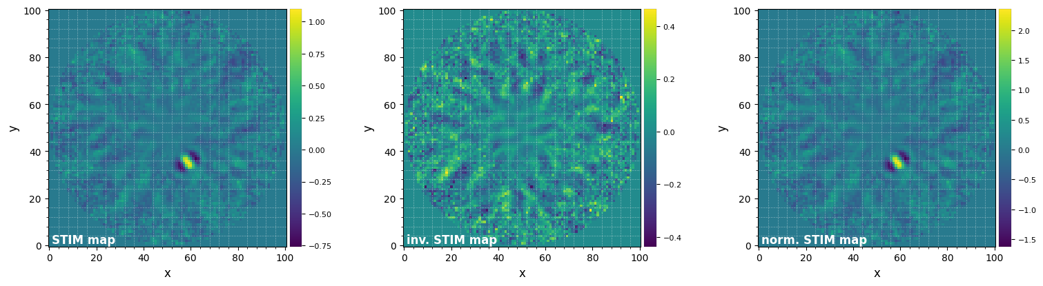
Any value larger than unity in the normalized STIM map is therefore expected to be significant. This can be visualized by thresholding the normalized STIM map.

thr_stim_map = norm_stim_map.copy()
thr_stim_map[np.where(thr_stim_map<1)]=0

Beta Pic b is considered significant with the above criterion, although no extended disc structure is detected:

plot_frames((pca_img, thr_stim_map), grid=True,
            label=('PCA image (npc=15)', 'thresholded norm. STIM map'))

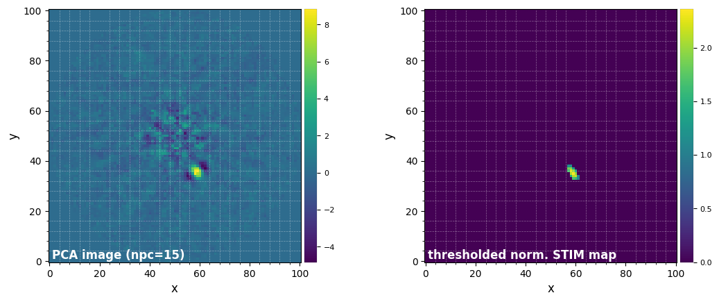
Note that in presence of azimuthally extended disc signals, the above criterion may still be too conservative to capture all disc signals present in the image - as these signals may also show up in the inverse STIM map and even dominate the maximum inverse STIM map values. Differential imaging strategies relying on other sources of diversity are required to identify azimuthally extended signals (e.g. RDI, SDI or PDI).

Answer 4.1: When test apertures include disc signal, the mean flux \(\bar{x}_2\) will be higher and/or the noise level will be overestimated (if the extended signal does not cover all apertures), hence leading in both cases to an underestimated S/N ratio of authentic disc signals. The above definition is therefore only relevant for point source detection.

Answer 4.2: With enough follow-up observations one can monitor the relative astrometry of the companion candidate with respect to the star, and compare it to the proper motion of the star (typically known to good precision thanks to Gaia for nearby stars). A background object (much further away) is expected to have a significantly different (typically much smaller) proper motion than the target. In absence of follow-up observations, a first statistical argument can be made based on the

separation of the companion candidate and the number density of background objects in that area of the sky - this can be estimated with VIP’s vip.stats.bkg_star_proba routine combined with the help of a Galactic model (e.g. TRILEGAL or Besançon model).

4.3. Automatic detection function

Let’s try the detection function in the metrics module. This is a computer vision blob-detection method based on the Laplacian of Gaussian filter (http://scikit-image.org/docs/dev/api/skimage.feature.html#skimage.feature.blob_log).

Provided a post-processed frame, the FWHM in pixels and a PSF (i.e. what a planet should look like), this function can return the position of point-like sources in the image. Take a look at the help/docstring for a detailed explanation of the function. Depending on the mode the results can be different. A S/N minimum criterion can be provided with snr_thresh.

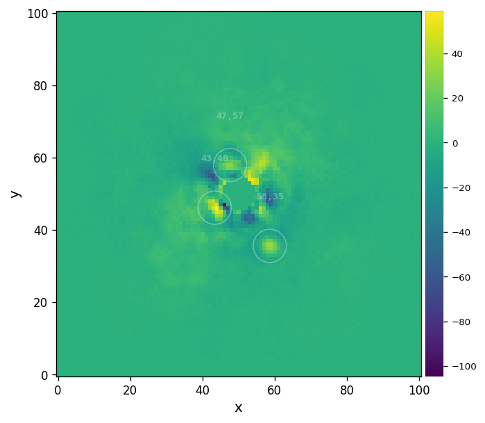
Let’s try it on the median-ADI and annular PCA images obtained on the Beta Pic b dataset:

fr_adi = median_sub(cube, angs)
detection(fr_adi, fwhm=fwhm_naco, psf=psfn, debug=False, mode='log', snr_thresh=5,
          bkg_sigma=5, matched_filter=False)

――――――――――――――――――――――――――――――――――――――――――――――――――――――――――――――――――――――――――――――――
Starting time: 2022-05-12 12:28:32
――――――――――――――――――――――――――――――――――――――――――――――――――――――――――――――――――――――――――――――――
Median psf reference subtracted
Done derotating and combining
Running time:  0:00:01.133273
――――――――――――――――――――――――――――――――――――――――――――――――――――――――――――――――――――――――――――――――
Blobs found: 3
 ycen   xcen
------ ------
46.130   43.396
35.555   58.654
57.920   47.674

――――――――――――――――――――――――――――――――――――――――――――――――――――――――――――――――――――――――――――――――
X,Y = (43.4,46.1)
S/N constraint NOT fulfilled (S/N = 1.585)

――――――――――――――――――――――――――――――――――――――――――――――――――――――――――――――――――――――――――――――――
X,Y = (58.7,35.6)
S/N constraint NOT fulfilled (S/N = 2.696)

――――――――――――――――――――――――――――――――――――――――――――――――――――――――――――――――――――――――――――――――
X,Y = (47.7,57.9)
S/N constraint NOT fulfilled (S/N = 0.928)
――――――――――――――――――――――――――――――――――――――――――――――――――――――――――――――――――――――――――――――――

	y	x

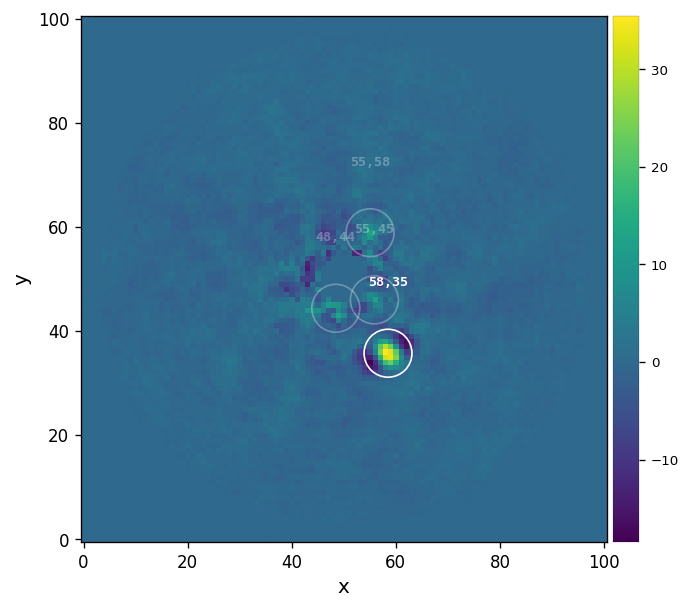
Planet b is highlighted but with rather small S/N (~2). We note that a number of other much less convicing blobs are also highlighted. Let’s try the frame obtained with annular PCA:

fr_pca = pca_annular(cube, angs, ncomp=7)
detection(fr_pca, fwhm=fwhm_naco, psf=psfn, bkg_sigma=5, debug=False, mode='log',
          snr_thresh=5, plot=True, verbose=True)

――――――――――――――――――――――――――――――――――――――――――――――――――――――――――――――――――――――――――――――――
Starting time: 2022-05-12 12:28:33
――――――――――――――――――――――――――――――――――――――――――――――――――――――――――――――――――――――――――――――――
N annuli = 12, FWHM = 4.000
PCA per annulus (or annular sectors):
Ann 1    PA thresh: 11.42    Ann center:   2    N segments: 1
Done PCA with lapack for current annulus
Running time:  0:00:00.032089
――――――――――――――――――――――――――――――――――――――――――――――――――――――――――――――――――――――――――――――――
Ann 2    PA thresh:  6.94    Ann center:   6    N segments: 1
Done PCA with lapack for current annulus
Running time:  0:00:00.333219
――――――――――――――――――――――――――――――――――――――――――――――――――――――――――――――――――――――――――――――――
Ann 3    PA thresh:  6.04    Ann center:  10    N segments: 1
Done PCA with lapack for current annulus
Running time:  0:00:00.481398
――――――――――――――――――――――――――――――――――――――――――――――――――――――――――――――――――――――――――――――――
Ann 4    PA thresh:  5.65    Ann center:  14    N segments: 1
Done PCA with lapack for current annulus
Running time:  0:00:00.607929
――――――――――――――――――――――――――――――――――――――――――――――――――――――――――――――――――――――――――――――――
Ann 5    PA thresh:  5.44    Ann center:  18    N segments: 1
Done PCA with lapack for current annulus
Running time:  0:00:00.758692
――――――――――――――――――――――――――――――――――――――――――――――――――――――――――――――――――――――――――――――――
Ann 6    PA thresh:  5.30    Ann center:  22    N segments: 1
Done PCA with lapack for current annulus
Running time:  0:00:00.938450
――――――――――――――――――――――――――――――――――――――――――――――――――――――――――――――――――――――――――――――――
Ann 7    PA thresh:  5.21    Ann center:  26    N segments: 1
Done PCA with lapack for current annulus
Running time:  0:00:01.132032
――――――――――――――――――――――――――――――――――――――――――――――――――――――――――――――――――――――――――――――――
Ann 8    PA thresh:  5.14    Ann center:  30    N segments: 1
Done PCA with lapack for current annulus
Running time:  0:00:01.315886
――――――――――――――――――――――――――――――――――――――――――――――――――――――――――――――――――――――――――――――――
Ann 9    PA thresh:  5.08    Ann center:  34    N segments: 1
Done PCA with lapack for current annulus
Running time:  0:00:01.485998
――――――――――――――――――――――――――――――――――――――――――――――――――――――――――――――――――――――――――――――――
Ann 10    PA thresh:  5.04    Ann center:  38    N segments: 1
Done PCA with lapack for current annulus
Running time:  0:00:01.706212
――――――――――――――――――――――――――――――――――――――――――――――――――――――――――――――――――――――――――――――――
Ann 11    PA thresh:  5.01    Ann center:  42    N segments: 1
Done PCA with lapack for current annulus
Running time:  0:00:01.875746
――――――――――――――――――――――――――――――――――――――――――――――――――――――――――――――――――――――――――――――――
Ann 12    PA thresh:  5.09    Ann center:  45    N segments: 1
Done PCA with lapack for current annulus
Running time:  0:00:02.086179
――――――――――――――――――――――――――――――――――――――――――――――――――――――――――――――――――――――――――――――――
Done derotating and combining.
Running time:  0:00:03.195348
――――――――――――――――――――――――――――――――――――――――――――――――――――――――――――――――――――――――――――――――
Blobs found: 4
 ycen   xcen
------ ------
35.703   58.491
58.856   55.039
45.943   55.871
44.344   48.461

――――――――――――――――――――――――――――――――――――――――――――――――――――――――――――――――――――――――――――――――
X,Y = (58.5,35.7)
――――――――――――――――――――――――――――――――――――――――――――――――――――――――――――――――――――――――――――――――
Coords of chosen px (X,Y) = 58.5, 35.7
Flux in a centered 1xFWHM circular aperture = 364.937
Central pixel S/N = 10.052
――――――――――――――――――――――――――――――――――――――――――――――――――――――――――――――――――――――――――――――――
Inside a centered 1xFWHM circular aperture:
Mean S/N (shifting the aperture center) = 8.353
Max S/N (shifting the aperture center) = 10.575
stddev S/N (shifting the aperture center) = 1.773


――――――――――――――――――――――――――――――――――――――――――――――――――――――――――――――――――――――――――――――――
X,Y = (55.0,58.9)
S/N constraint NOT fulfilled (S/N = 2.645)

――――――――――――――――――――――――――――――――――――――――――――――――――――――――――――――――――――――――――――――――
X,Y = (55.9,45.9)
S/N constraint NOT fulfilled (S/N = 1.460)

――――――――――――――――――――――――――――――――――――――――――――――――――――――――――――――――――――――――――――――――
X,Y = (48.5,44.3)
S/N constraint NOT fulfilled (S/N = 2.173)
――――――――――――――――――――――――――――――――――――――――――――――――――――――――――――――――――――――――――――――――

	y	x
0	35.702519	58.491348

We see from these tests that one should take the results obtained by this automatic detection algorithm with a pinch of salt (see. e.g the signals at the edge of the inner mask). It is unlikely to detect point sources better then can be inferred from visual inspection by human eyes. Much more advanced machine learning techniques should be used to infer the presence of companions that cannot be detected from visual inspection of the final image, and with low false positive fraction (see e.g. Gomez Gonzalez et al. 2018).

4.4. Throughput and contrast curves

4.4.1. Throughput

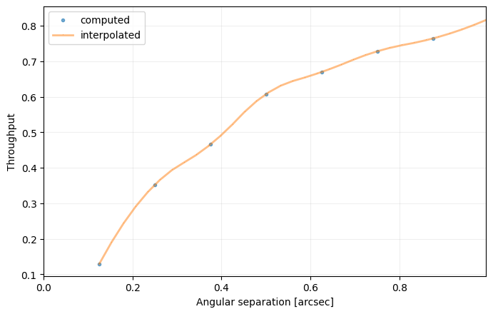
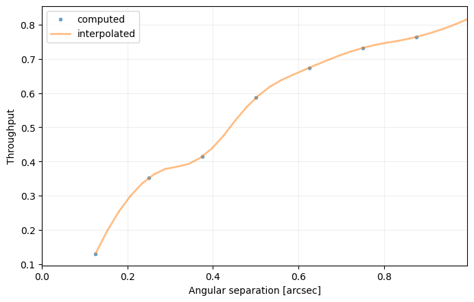
VIP allows to measure the throughput of its algorithms by injecting fake companions. The throughput gives us an idea of how much the algorithm subtracts or biases the signal from companions, as a function of the distance from the center (high throughput = low amount of self-subtraction). Let’s assess it for our toy datacube. The relevant function is throughput in the metrics module.

In order to measure reliable throughput and contrast curves, one first need to subtract from the data all real companions.

We’ll see in Tutorial 5. how to obtain reliable estimates on the parameters of directly imaged companions (radial separation, azimuth and flux). Let’s assume we have inferred these parameters. It is only a matter of calling the cube_planet_free function in the fm module:

r_b =  0.452/pxscale_naco # Absil et al. (2013)
theta_b = 211.2+90 # Absil et al. (2013) - note the VIP convention is to measure angles from positive x axis
f_b = 648.2

cube_emp = cube_planet_free([(r_b, theta_b, f_b)], cube, angs, psfn=psfn)

Let’s double check the planet was efficiently removed:

pca_emp = pca(cube_emp, angs, ncomp=12, verbose=False)
plot_frames(pca_emp, axis=False)

Let’s now compute the throughput with the empty cube:

res_thr = throughput(cube_emp, angs, psfn, fwhm_naco, ncomp=15,
                     algo=pca, nbranch=1, full_output=True)

――――――――――――――――――――――――――――――――――――――――――――――――――――――――――――――――――――――――――――――――
Starting time: 2022-05-12 12:28:38
――――――――――――――――――――――――――――――――――――――――――――――――――――――――――――――――――――――――――――――――
Cube without fake companions processed with pca
Running time:  0:00:01.129060
――――――――――――――――――――――――――――――――――――――――――――――――――――――――――――――――――――――――――――――――
Measured annulus-wise noise in resulting frame
Running time:  0:00:01.148820
――――――――――――――――――――――――――――――――――――――――――――――――――――――――――――――――――――――――――――――――
Flux in 1xFWHM aperture: 1.000
Fake companions injected in branch 1 (pattern 1/3)
Running time:  0:00:01.187973
――――――――――――――――――――――――――――――――――――――――――――――――――――――――――――――――――――――――――――――――
Cube with fake companions processed with pca
Measuring its annulus-wise throughput
Running time:  0:00:02.311214
――――――――――――――――――――――――――――――――――――――――――――――――――――――――――――――――――――――――――――――――
Fake companions injected in branch 1 (pattern 2/3)
Running time:  0:00:02.340897
――――――――――――――――――――――――――――――――――――――――――――――――――――――――――――――――――――――――――――――――
Cube with fake companions processed with pca
Measuring its annulus-wise throughput
Running time:  0:00:03.468227
――――――――――――――――――――――――――――――――――――――――――――――――――――――――――――――――――――――――――――――――
Fake companions injected in branch 1 (pattern 3/3)
Running time:  0:00:03.490540
――――――――――――――――――――――――――――――――――――――――――――――――――――――――――――――――――――――――――――――――
Cube with fake companions processed with pca
Measuring its annulus-wise throughput
Running time:  0:00:04.607704
――――――――――――――――――――――――――――――――――――――――――――――――――――――――――――――――――――――――――――――――
Finished measuring the throughput in 1 branches
Running time:  0:00:04.609510
――――――――――――――――――――――――――――――――――――――――――――――――――――――――――――――――――――――――――――――――

figure(figsize=(6,3))
plot(res_thr[3], res_thr[0][0,:], 'o-', alpha=0.5)
ylabel('throughput')
xlabel('separation in pixels')

Text(0.5, 0, 'separation in pixels')

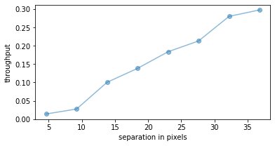
Question 4.3: Why does the throughput increase with radial separation?

Let’s compare this with the annular PCA result:

res_thr2 = throughput(cube_emp, angs, psfn, fwhm_naco, algo=pca_annular, nbranch=1, verbose=False,
                      full_output=True, ncomp=10, radius_int=int(fwhm_naco),
                      delta_rot=1, asize=6)

figure(figsize=(6,3))
plot(res_thr[3], res_thr[0][0,:], 'o-', label='PCA', alpha=0.5)
plot(res_thr2[3], res_thr2[0][0,:], 'o-', label='annular PCA', alpha=0.5)
ylabel('throughput')
xlabel('separation in pixels')
_ = legend(loc='best')

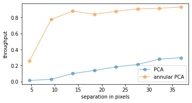
We clearly see the gain in throughput by applying a parallactic angle rejection in our annular PCA processing. For a sequence with more field rotation, the delta_rot value could be increased to further increase the throughput.

Answer 4.3: For a given parallactic angle threshold (or lack thereof in standard pca.pca), there is more linear motion of the field radially outward, resulting in less self-subtraction of any putative planet.

4.4.2. Contrast curves

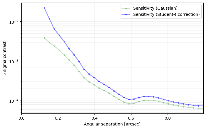
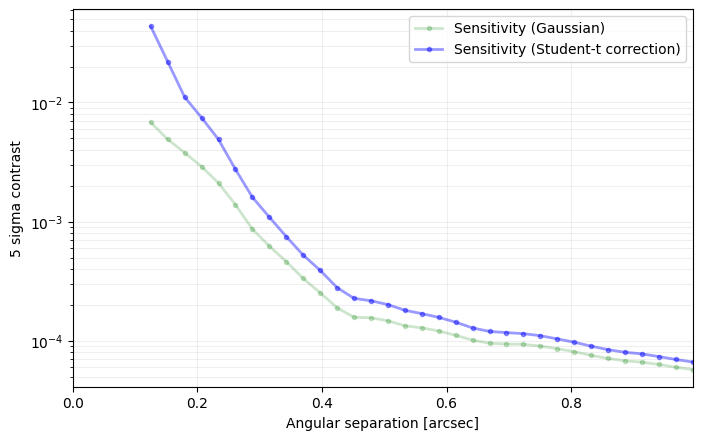
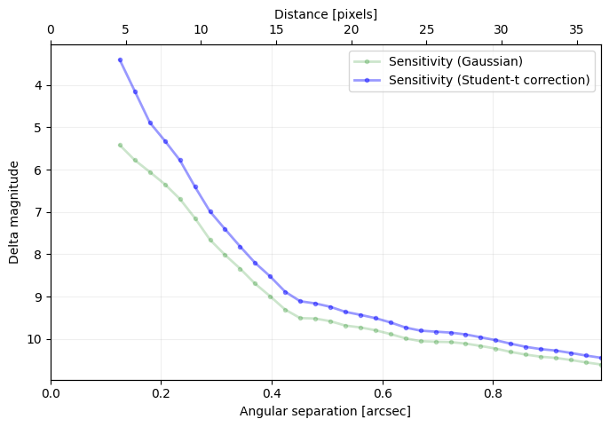
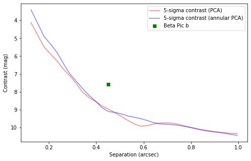
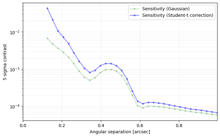
Now let’s see how to generate 5-sigma contrast curves for ADI data using the contrast_curve function. The contrast curve shows the achieved contrast (i.e. how much fainter than the star a companion can be detected) as a function of radius, for a given datacube post-processed with a given algorithm.

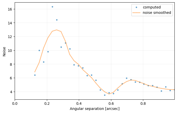
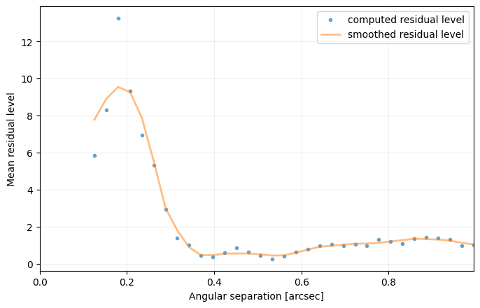
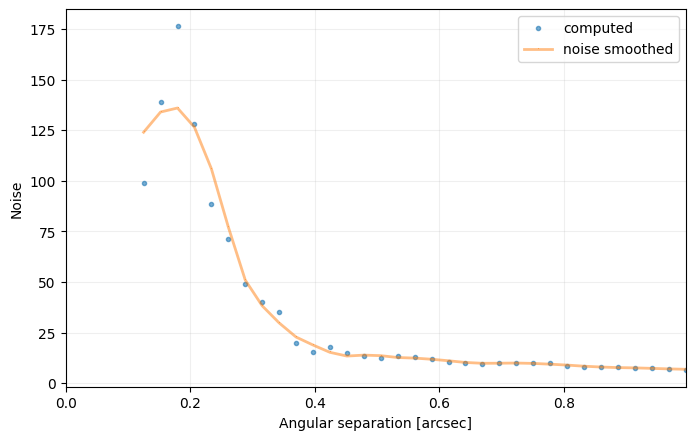
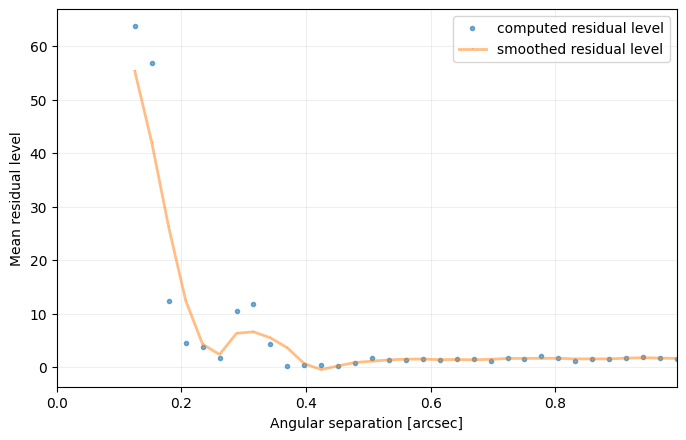
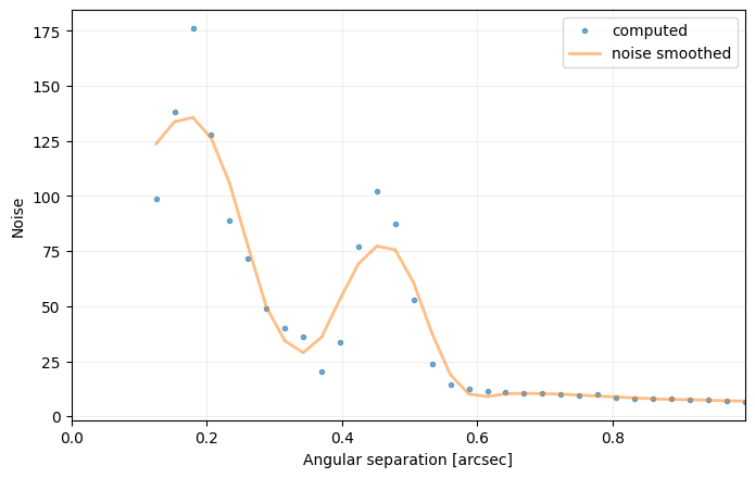
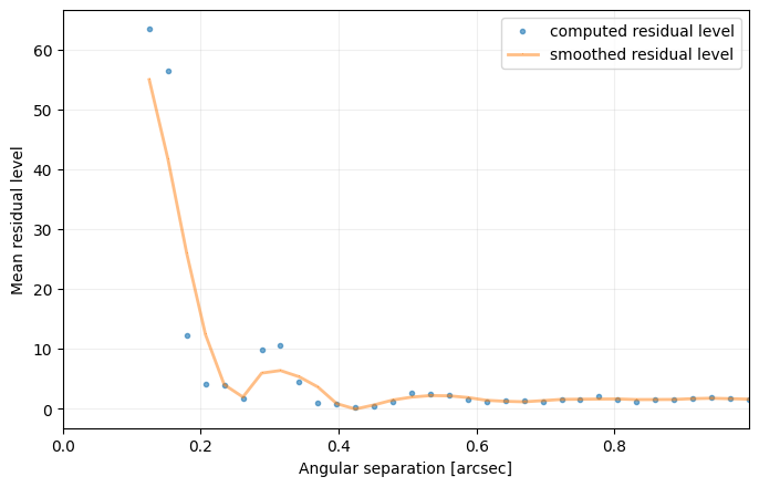
The contrast curve takes into account both the noise level in the final image and the algorithmic throughput (previous subsection). The noise level is used to infer the signal required for the S/N to achieve a 5-sigma significance at each radial separation, as calculated in Section 4.2. Note that sigma is an input parameter such that the contrast curve can also be calculated for e.g. 1 or 3 \(\sigma\). Let’s set it to 5:

nsig=5

Among other parameters of the contrast_curve function, algo takes any function in VIP for model PSF subtraction, and optional parameters of the algo can also be passed as regular parameters of contrast_curve. Parameter starphot sets the flux of the star. The latter was obtained from the non-coronagraphic PSF before normalization:

starphot = 764939.6

In the example below, we’ll first calculate the contrast curve obtained with full-frame PCA, and then with PCA in concentric annuli with a PA threshold.

cc_1 = contrast_curve(cube_emp, angs, psfn, fwhm=fwhm_naco, pxscale=pxscale_naco, starphot=starphot,
                      sigma=nsig, nbranch=1, algo=pca, ncomp=9, debug=True)

――――――――――――――――――――――――――――――――――――――――――――――――――――――――――――――――――――――――――――――――
Starting time: 2022-05-12 12:28:52
――――――――――――――――――――――――――――――――――――――――――――――――――――――――――――――――――――――――――――――――
ALGO : pca, FWHM = 4.603450563658683, # BRANCHES = 1, SIGMA = 5, STARPHOT = 764939.6
――――――――――――――――――――――――――――――――――――――――――――――――――――――――――――――――――――――――――――――――
Finished the throughput calculation
Running time:  0:00:04.559482
――――――――――――――――――――――――――――――――――――――――――――――――――――――――――――――――――――――――――――――――

cc_2 = contrast_curve(cube_emp, angs, psfn, fwhm=fwhm_naco, pxscale=pxscale_naco, starphot=starphot,
                      sigma=nsig, nbranch=1, delta_rot=0.5, algo=pca_annular, ncomp=8,
                      radius_int=int(fwhm_naco), debug=True)

――――――――――――――――――――――――――――――――――――――――――――――――――――――――――――――――――――――――――――――――
Starting time: 2022-05-12 12:28:57
――――――――――――――――――――――――――――――――――――――――――――――――――――――――――――――――――――――――――――――――
ALGO : pca_annular, FWHM = 4.603450563658683, # BRANCHES = 1, SIGMA = 5, STARPHOT = 764939.6
――――――――――――――――――――――――――――――――――――――――――――――――――――――――――――――――――――――――――――――――
Finished the throughput calculation
Running time:  0:00:11.174366
――――――――――――――――――――――――――――――――――――――――――――――――――――――――――――――――――――――――――――――――

Question 4.4: Considering the hard encoded planet parameters and stellar flux provided above, where would Beta Pic b sit in this contrast curve?

Question 4.5: If a companion is present in the datacube, how do you expect it to affect the contrast curve? In other words what would happen if cube was provided to contrast_curve instead of cube_emp?

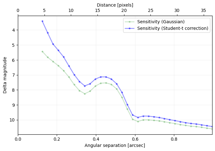
Answer 4.4: As illustrated below.

figure(figsize=(8,5))
plt.plot(cc_1['distance']*pxscale_naco,
         -2.5*np.log10(cc_1['sensitivity_student']),
         'r-', label='{}-sigma contrast (PCA)'.format(nsig), alpha=0.5)
plt.plot(cc_2['distance']*pxscale_naco,
         -2.5*np.log10(cc_2['sensitivity_student']),
         'b-', label='{}-sigma contrast (annular PCA)'.format(nsig), alpha=0.5)
r_b = 16.583
plt.plot(r_b*pxscale_naco,
         -2.5*np.log10(700./starphot), 'gs', label='Beta Pic b')
plt.gca().invert_yaxis()
ylabel('Contrast (mag)')
xlabel('Separation (arcsec)')
_ = legend(loc='best')
plt.show()

Answer 4.5: It would artificially increase the estimated contrast at the radial separation of the companion (creating a bump in the curve) - as it would be considered as extra noise. Illustration below:

cc_not_emp = contrast_curve(cube, angs, psfn, fwhm=fwhm_naco, pxscale=pxscale_naco, starphot=starphot,
                            sigma=nsig, nbranch=1, delta_rot=0.5, algo=pca_annular, ncomp=8,
                            radius_int=int(fwhm_naco), debug=True)

――――――――――――――――――――――――――――――――――――――――――――――――――――――――――――――――――――――――――――――――
Starting time: 2022-05-12 12:29:09
――――――――――――――――――――――――――――――――――――――――――――――――――――――――――――――――――――――――――――――――
ALGO : pca_annular, FWHM = 4.603450563658683, # BRANCHES = 1, SIGMA = 5, STARPHOT = 764939.6
――――――――――――――――――――――――――――――――――――――――――――――――――――――――――――――――――――――――――――――――
Finished the throughput calculation
Running time:  0:00:11.389965
――――――――――――――――――――――――――――――――――――――――――――――――――――――――――――――――――――――――――――――――

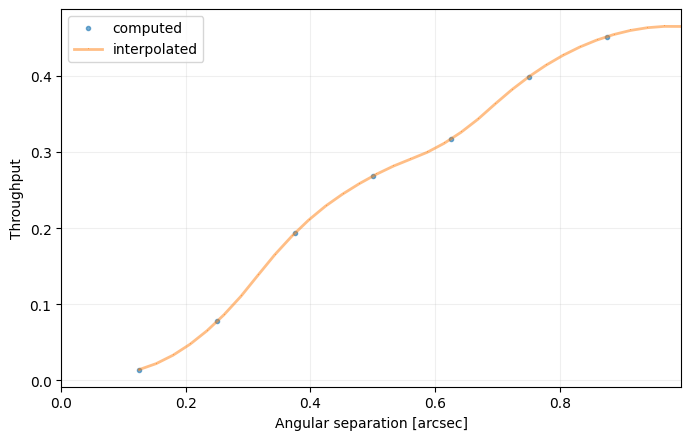
4.5. Completeness curves and maps

4.5.1. Completeness curves

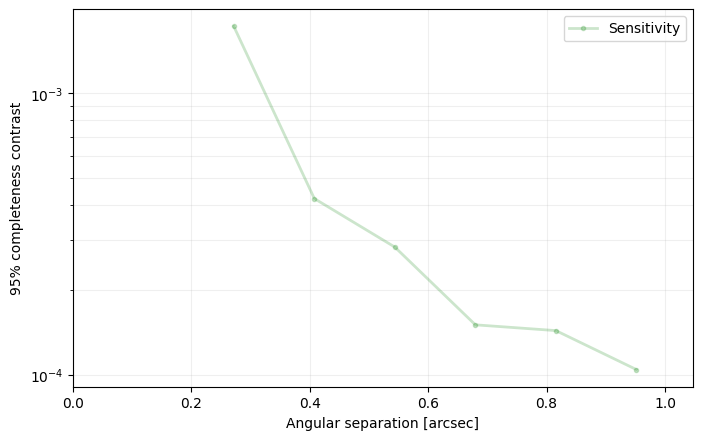
VIP allows the calculation of completeness curves, as implemented in Dahlqvist et al. (2021) following the framework introduced in Jensen-Clem et al. (2018).

These are contrast curves corresponding to a given completeness level (e.g. 95%) and one false positive in the full frame. In other words, the 95% completeness curve corresponds to the contrast at which a given companion would be recovered 95% of the time (19/20 true positives).

Setting an_dist to None produces a contrast curve spanning 2 FWHM in radius to half the size of the provided cube images minus half of the PSF frame, with a step of 5 pixels.

crop_sz = 15
if psf.shape[-1]>crop_sz:
    psf = frame_crop(psf, crop_sz)
an_dist, comp_curve = completeness_curve(cube_emp, angs, psf, fwhm_naco, pca, an_dist=np.arange(10,40,5),
                                         pxscale=pxscale_naco, ini_contrast=None, starphot=starphot,
                                         plot=True, nproc=None, algo_dict={'ncomp':3, 'imlib':'opencv'})

New shape: (15, 15)
Contrast curve not provided => will be computed first...
――――――――――――――――――――――――――――――――――――――――――――――――――――――――――――――――――――――――――――――――
Starting time: 2022-05-12 12:29:21
――――――――――――――――――――――――――――――――――――――――――――――――――――――――――――――――――――――――――――――――
ALGO : pca, FWHM = 4.603450563658683, # BRANCHES = 1, SIGMA = 3, STARPHOT = 764939.6
――――――――――――――――――――――――――――――――――――――――――――――――――――――――――――――――――――――――――――――――
Finished the throughput calculation
Running time:  0:00:00.448024
――――――――――――――――――――――――――――――――――――――――――――――――――――――――――――――――――――――――――――――――
Calculating initial SNR map with no injected companion...
*** Calculating contrast at r = 10 ***
Found contrast level for first TP detection: 0.0015327681548457951
Found lower and upper bounds of sought contrast: [0.0015327681548457951, 0.0022991522322686926]
=> found final contrast for 95.0% completeness: 0.0017243641742015195
*** Calculating contrast at r = 15 ***
Found contrast level for first TP detection: 0.0003616123294953311
Found lower and upper bounds of sought contrast: [0.0003616123294953311, 0.0005424184942429967]
=> found final contrast for 95.0% completeness: 0.0004221639482406645
*** Calculating contrast at r = 20 ***
Found contrast level for first TP detection: 0.0002071523791812666
Found lower and upper bounds of sought contrast: [0.0002071523791812666, 0.0003107285687718999]
=> found final contrast for 95.0% completeness: 0.00028393862916889663
*** Calculating contrast at r = 25 ***
Found contrast level for first TP detection: 0.00011326538009746645
Found lower and upper bounds of sought contrast: [0.00011326538009746645, 0.00016989807014619967]
=> found final contrast for 95.0% completeness: 0.00015042208803844033
*** Calculating contrast at r = 30 ***
Found contrast level for first TP detection: 9.565560076278946e-05
Found lower and upper bounds of sought contrast: [9.565560076278946e-05, None]
=> found final contrast for 95.0% completeness: 0.0001434834011441842
*** Calculating contrast at r = 35 ***
Found contrast level for first TP detection: 8.217772195037159e-05
Found lower and upper bounds of sought contrast: [8.217772195037159e-05, 0.0001232665829255574]
=> found final contrast for 95.0% completeness: 0.00010435646573372887

4.5.2. Completeness maps

One can also compute completeness maps, considering the dependency of the contrast on both radius and completeness. Since this is a very slow process (even slower than the completeness curve), we will limit it to only one of the radii tested for the completeness curves, and set the initial contrast (ini_contrast) to the output of the completeness_curve function at that radius:

n_fc = 20
test_an_dist = 25 # tested radial distance

# initial contrast set to value found in completeness curve
idx = np.where(an_dist == test_an_dist)[0]
ini_contrast = comp_curve[idx]

an_dist, comp_levels, contrasts = completeness_map(cube_emp, angs, psf, fwhm_naco, pca, an_dist=[test_an_dist],
                                                   n_fc=n_fc, ini_contrast=ini_contrast, starphot=starphot,
                                                   nproc=None, algo_dict={'ncomp':3, 'imlib':'opencv'})

Starting annulus 25
Lower bound (5%) found: 1.1294395289843065e-05
Upper bound (95%) found: 0.00015042208803844033
Data point 0.15 found. Still 14 data point(s) missing
Data point 0.25 found. Still 13 data point(s) missing
Data point 0.3 found. Still 11 data point(s) missing
Data point 0.4 found. Still 10 data point(s) missing
Data point 0.45 found. Still 9 data point(s) missing
Data point 0.55 found. Still 8 data point(s) missing
Data point 0.65 found. Still 6 data point(s) missing
Data point 0.7 found. Still 5 data point(s) missing
Data point 0.75 found. Still 4 data point(s) missing
Data point 0.9 found. Still 1 data point(s) missing

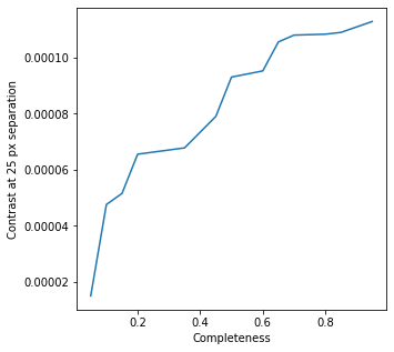
Let’s plot the achieved contrast as a function of the assumed completeness ratio, at a radial separation of 25 px:

fig = plt.figure(figsize = [5,5])
plt.plot(comp_levels, contrasts[0,:])
plt.xlabel("Completeness")
plt.ylabel("Contrast at {} px separation".format(test_an_dist))
plt.show()