5. ADI forward modeling of point sources
Authors: Valentin Christiaens and Carlos Alberto Gomez GonzalezSuitable for VIP v1.0.0 onwardsLast update: 2022/09/21
Table of contents
- 5.1. Loading ADI data
- 5.2. Generating and injecting synthetic planets
- 5.3. Flux and position estimation with NEGFC
This tutorial shows:
- how to generate and inject fake companions in a cube;
- how to estimate the astrometry and photometry of a directly imaged companion, and associated uncertainties.
Let’s first import a couple of external packages needed in this tutorial:
[1]:
%matplotlib inline
from hciplot import plot_frames, plot_cubes
from matplotlib.pyplot import *
from matplotlib import pyplot as plt
import numpy as np
from packaging import version
In the following box we import all the VIP routines that will be used in this tutorial. The path to some routines has changed between versions 1.0.3 and 1.1.0, which saw a major revamp of the modular architecture, hence the if statements.
[2]:
import vip_hci as vip
vvip = vip.__version__
print("VIP version: ", vvip)
if version.parse(vvip) < version.parse("1.0.0"):
    msg = "Please upgrade your version of VIP"
    msg+= "It should be 1.0.0 or above to run this notebook."
    raise ValueError(msg)
elif version.parse(vvip) <= version.parse("1.0.3"):
    from vip_hci.conf import VLT_NACO
    from vip_hci.metrics import cube_inject_companions
    from vip_hci.negfc import (confidence, firstguess, mcmc_negfc_sampling, show_corner_plot, show_walk_plot,
                               speckle_noise_uncertainty)
    from vip_hci.pca import pca, pca_annular, pca_annulus, pca_grid
else:
    from vip_hci.config import VLT_NACO
    from vip_hci.fm import (confidence, cube_inject_companions, cube_planet_free, firstguess, mcmc_negfc_sampling,
                            normalize_psf, show_corner_plot, show_walk_plot, speckle_noise_uncertainty)
    from vip_hci.psfsub import median_sub, pca, pca_annular, pca_annulus, pca_grid

# common to all versions:
from vip_hci.fits import open_fits, write_fits, info_fits
from vip_hci.metrics import contrast_curve, detection, significance, snr, snrmap, throughput
from vip_hci.preproc import frame_crop
from vip_hci.var import fit_2dgaussian, frame_center
VIP version: 1.2.4
5.1. Loading ADI data
In the ‘dataset’ folder of the VIP_extras repository you can find a toy ADI (Angular Differential Imaging) cube and a NACO point spread function (PSF) to demonstrate the capabilities of VIP. This is an L’-band VLT/NACO dataset of beta Pictoris published in Absil et al. (2013) obtained using the Annular Groove Phase Mask (AGPM) Vortex coronagraph. The sequence has been heavily sub-sampled temporarily to make it
smaller. The frames were also cropped to the central 101x101 area. In case you want to plug-in your cube just change the path of the following cells.
More info on this dataset, and on opening and visualizing fits files with VIP in general, is available in Tutorial 1. Quick start.
Let’s load the data:
[3]:
psfnaco = '../datasets/naco_betapic_psf.fits'
cubename = '../datasets/naco_betapic_cube_cen.fits'
angname = '../datasets/naco_betapic_pa.fits'

cube = open_fits(cubename)
psf = open_fits(psfnaco)
pa = open_fits(angname)
Fits HDU-0 data successfully loaded. Data shape: (61, 101, 101)
Fits HDU-0 data successfully loaded. Data shape: (39, 39)
Fits HDU-0 data successfully loaded. Data shape: (61,)
[4]:
derot_off = 104.84 # NACO derotator offset for this observation (Absil et al. 2013)
TN = -0.45         # Position angle of true north for NACO at the epoch of observation (Absil et al. 2013)

angs = pa+derot_off+TN
Let’s measure the FWHM by fitting a 2D Gaussian to the core of the unsaturated non-coronagraphic PSF:
[5]:
%matplotlib inline
DF_fit = fit_2dgaussian(psf, crop=True, cropsize=9, debug=True, full_output=True)
FWHM_y = 4.733218722257407
FWHM_x = 4.473682405059958

centroid y = 19.006680059041216
centroid x = 18.999424475165455
centroid y subim = 4.006680059041214
centroid x subim = 3.9994244751654535

amplitude = 0.10413004853269707
theta = -34.08563676836685
[6]:
fwhm_naco = np.mean([DF_fit['fwhm_x'],DF_fit['fwhm_y']])
print(fwhm_naco)
4.603450563658683
Let’s normalize the flux to one in a 1xFWHM aperture and crop the PSF array:
[7]:
psfn = normalize_psf(psf, fwhm_naco, size=19, imlib='ndimage-fourier')
Flux in 1xFWHM aperture: 1.228
[8]:
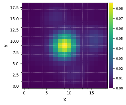
plot_frames(psfn, grid=True, size_factor=4)
Let’s finally define the pixel scale for NACO (L’ band), which we get from a dictionary stored in the config subpackage:
[9]:
pxscale_naco = VLT_NACO['plsc']
print(pxscale_naco, "arcsec/px")
0.02719 arcsec/px
5.2. Generating and injecting synthetic planets
We first select an image library imlib for image operations (shifts, rotations) and associated interpolation order. ‘vip-fft’ is more accurate, but ‘skimage’ is faster, and ‘opencv’ even faster - see Tutorial 7 for more details.
[10]:
imlib_rot = 'opencv' #'skimage'
interpolation='lanczos4' #'biquintic'
The cube_inject_companions function in the fm module (VIP versions >= 1.1.0) makes the injection of fake companions at arbitrary fluxes and locations very easy. The normalized non-coronagraphic PSF should be provided for the injection. If the user does not have access to an observed PSF, the create_synth_psf from the var module can be used to create synthetic ones (based on 2D Gaussian, Moffat or Airy models).
Some procedures, e.g. the negative fake companion technique and the contrast curve generation, heavily rely on the injection of fake companions. The coordinates for the injection should be provided in the derotated image, while the actual injection occurs in the images of the input cube, i.e. in the rotated field.
[11]:
rad_fc = 30.5
theta_fc = 240
flux_fc = 400.

gt = [rad_fc, theta_fc, flux_fc]
[12]:
cubefc = cube_inject_companions(cube, psf_template=psfn, angle_list=angs, flevel=flux_fc, plsc=pxscale_naco,
                                rad_dists=[rad_fc], theta=theta_fc, n_branches=1,
                                imlib=imlib_rot, interpolation=interpolation)
Let’s set the corresponding cartesian coordinates:
[13]:
cy, cx = frame_center(cube[0])
x_fc = cx + rad_fc*np.cos(np.deg2rad(theta_fc))
y_fc = cy + rad_fc*np.sin(np.deg2rad(theta_fc))

xy_test = (x_fc, y_fc)
print('({:.1f}, {:.1f})'.format(xy_test[0],xy_test[1]))
(34.7, 23.6)
Let’s double-check the fake companion was injected at the right location, by post-processing the cube and checking the final image. Let’s use PCA, and infer the optimal \(n_{\rm pc}\) while we are at it - this will be useful for the next section.
[14]:
res_ann_opt = pca_grid(cubefc, angs, fwhm=fwhm_naco, range_pcs=(1,41,1), source_xy=xy_test, mode='annular',
                       annulus_width=4*fwhm_naco, imlib=imlib_rot, interpolation=interpolation,
                       full_output=True, plot=True)
――――――――――――――――――――――――――――――――――――――――――――――――――――――――――――――――――――――――――――――――
Starting time: 2022-05-04 13:37:46
――――――――――――――――――――――――――――――――――――――――――――――――――――――――――――――――――――――――――――――――
Done SVD/PCA with numpy SVD (LAPACK)
Running time:  0:00:00.057389
――――――――――――――――――――――――――――――――――――――――――――――――――――――――――――――――――――――――――――――――
Number of steps 41
Optimal number of PCs = 10, for S/N=13.415
――――――――――――――――――――――――――――――――――――――――――――――――――――――――――――――――――――――――――――――――
Coords of chosen px (X,Y) = 34.7, 23.6
Flux in a centered 1xFWHM circular aperture = 104.785
Central pixel S/N = 18.264
――――――――――――――――――――――――――――――――――――――――――――――――――――――――――――――――――――――――――――――――
Inside a centered 1xFWHM circular aperture:
Mean S/N (shifting the aperture center) = 13.415
Max S/N (shifting the aperture center) = 18.472
stddev S/N (shifting the aperture center) = 4.088
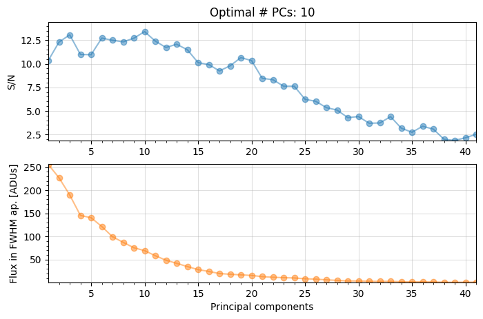
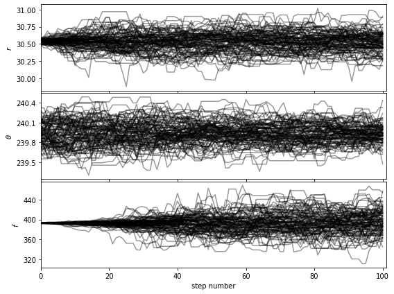
The grid search looking for the optimal number of principal components (npc) found that 10 principal components maximizes the S/N ratio of the injected fake companion.
[15]:
_, final_ann_opt, _, opt_npc_ann = res_ann_opt
[16]:
plot_frames(final_ann_opt, label='PCA-ADI annulus (opt. npc={:.0f})'.format(opt_npc_ann),
            dpi=100, vmin=-5, colorbar=True, circle=xy_test)

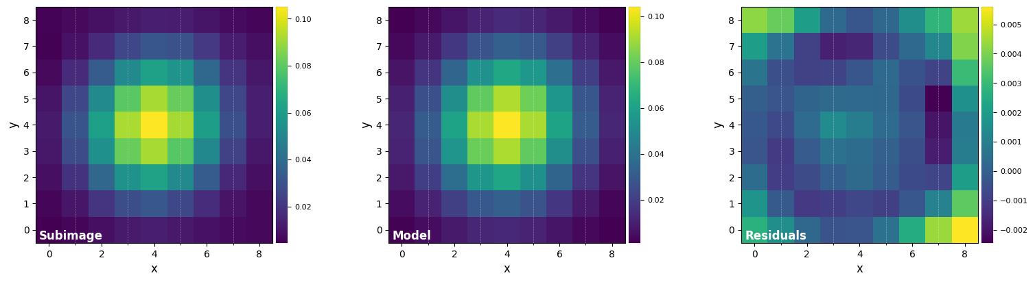
We can see that the fake companion was indeed injected at the requested location.
5.3. Flux and position estimation with NEGFC
When a companion candidate is detected, the next step is to characterize it, i.e. infer its exact position (astrometry) and flux (photometry).
Question 5.1: Why would a simple 2D Gaussian fit (as performed e.g. for the stellar PSF in Section 5.1) be inappropriate to extract the astrometry and photometry of a candidate companion?
VIP implements the Negative fake companion (NEGFC) technique for robust extraction of the position and flux of detected point-like sources. The technique can be summarized as follow (see full description in Wertz et al. 2017):
- Estimate the position and flux of the planet, from either the visual inspection of reduced images or a previous estimator (see ABC below).
- Scale (in flux) and shift the normalized off-axis PSF to remove the estimate from the input data cube.
- Process the cube with PCA in a single annulus encompassing the point source.
- Measure residuals in an aperture centered on the approximate location of the companion candidate.
- Iterate on the position and flux of the injected negative PSF (steps 2-4), until the absolute residuals in the aperture are minimized (i.e. the injected negative companion flux and the position match exactly that of the true companion).
Iterations between steps 2-4 can be performed in one of 3 ways - sorted in increasing computation time and accuracy:
- a grid search on the flux only, provided a fixed estimate of the position (implemented in the
firstguessfunction); - a Nelder-Mead simplex algorithm (
firstguessfunction with thesimplex=Trueoption); - an MCMC sampler, which has the advantage to also yield uncertainties on each of the parameters of the point source (
mcmc_negfc_samplingfunction).
Different figures of merit can be used for minimization of the residuals (Wertz et al. 2017; Christiaens et al. 2021):
where \(j \in {1,...,N}\), \(N\) is the total number of pixels contained in the circular aperture around the companion candidate, \(\mu\) and \(\sigma\) are the mean and standard deviation (\(N_{\rm resel}\) degrees of freedom) of pixel intensities in a truncated annulus at the radius of the companion candidate, but avoiding the azimuthal region encompassing the negative side lobes.
5.3.1. Nelder-Mead based optimization
With the function firstguess, we can obtain a first estimation of the flux and position by running A) a naive grid minimization (grid of values for the flux through parameter f_range), and B) a Nelder-mead based minimization (if the parameter simplex is set to True). The latter is done based on the preliminary guess of the grid minimization. The maximum number of iterations and error can be set with the parameter simplex_options as a dicitionary (see scipy.minimize function
for the Nelder-Mead options).
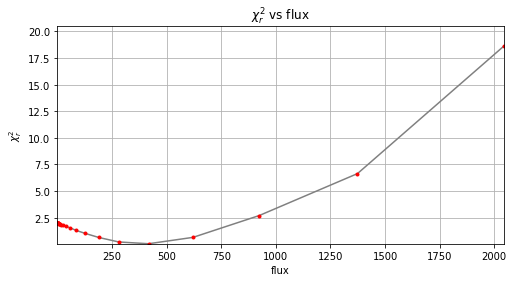
Fisrt we define the position of the sources by examining a flux frame or S/N map. planets_xy_coord takes a list or array of X,Y pairs like ((x1,y1),(x2,y2)…(x_n,y_n)). Let’s take the coordinates of the previously injected companion.
Let’s test the algorithm with different values for the # of PCs: 5 and 25.
[17]:
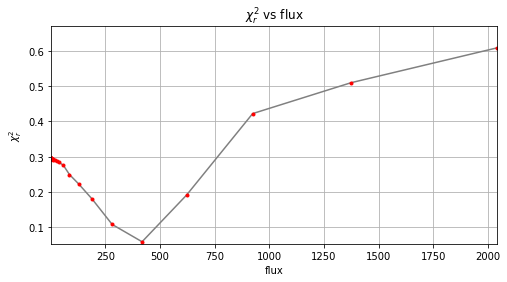
r_lo, theta_lo, f_lo = firstguess(cubefc, angs, psfn, ncomp=5, planets_xy_coord=[xy_test],
                                  fwhm=fwhm_naco, f_range=None, annulus_width=4*fwhm_naco,
                                  aperture_radius=2, simplex=True, imlib=imlib_rot,
                                  interpolation=interpolation, plot=True, verbose=True)
――――――――――――――――――――――――――――――――――――――――――――――――――――――――――――――――――――――――――――――――
Starting time: 2022-05-04 13:37:50
――――――――――――――――――――――――――――――――――――――――――――――――――――――――――――――――――――――――――――――――

――――――――――――――――――――――――――――――――――――――――――――――――――――――――――――――――――――――――――――――――
             Planet 0
――――――――――――――――――――――――――――――――――――――――――――――――――――――――――――――――――――――――――――――――

Planet 0: flux estimation at the position [34.749999999999986,23.58622518457463], running ...
Step | flux    | chi2r
1/30   0.100   1.975
2/30   0.149   1.974
3/30   0.221   1.974
4/30   0.329   1.972
5/30   0.489   1.971
6/30   0.728   1.969
7/30   1.083   1.965
8/30   1.610   1.960
9/30   2.395   1.953
10/30   3.562   1.942
11/30   5.298   1.926
12/30   7.880   1.902
13/30   11.721   1.866
14/30   17.433   1.813
15/30   25.929   1.733
16/30   38.566   1.615
17/30   57.362   1.446
18/30   85.317   1.216
19/30   126.896   0.926
20/30   188.739   0.554
21/30   280.722   0.179
22/30   417.532   0.047
23/30   621.017   0.777
24/30   923.671   3.817
25/30   1373.824   11.783

Planet 0: preliminary position guess: (r, theta)=(30.5, 240.0)
Planet 0: preliminary flux guess: 417.5
Planet 0: Simplex Nelder-Mead minimization, running ...
Planet 0: Success: True, nit: 97, nfev: 224, chi2r: 0.030578838959905028
message: Optimization terminated successfully.
Planet 0: simplex result: (r, theta, f)=(30.535, 239.976, 383.055) at
          (X,Y)=(34.72, 23.56)

 ――――――――――――――――――――――――――――――――――――――――――――――――――――――――――――――――――――――――――――――――
DONE !
 ――――――――――――――――――――――――――――――――――――――――――――――――――――――――――――――――――――――――――――――――
Running time:  0:00:23.468048
――――――――――――――――――――――――――――――――――――――――――――――――――――――――――――――――――――――――――――――――
[18]:
r_hi, theta_hi, f_hi = firstguess(cubefc, angs, psfn, ncomp=25, planets_xy_coord=[xy_test],
                                  fwhm=fwhm_naco, f_range=None, annulus_width=4*fwhm_naco,
                                  aperture_radius=2, imlib=imlib_rot, interpolation=interpolation,
                                  simplex=True, plot=True, verbose=True)
――――――――――――――――――――――――――――――――――――――――――――――――――――――――――――――――――――――――――――――――
Starting time: 2022-05-04 13:38:14
――――――――――――――――――――――――――――――――――――――――――――――――――――――――――――――――――――――――――――――――

――――――――――――――――――――――――――――――――――――――――――――――――――――――――――――――――――――――――――――――――
             Planet 0
――――――――――――――――――――――――――――――――――――――――――――――――――――――――――――――――――――――――――――――――

Planet 0: flux estimation at the position [34.749999999999986,23.58622518457463], running ...
Step | flux    | chi2r
1/30   0.100   0.295
2/30   0.149   0.295
3/30   0.221   0.295
4/30   0.329   0.295
5/30   0.489   0.295
6/30   0.728   0.295
7/30   1.083   0.295
8/30   1.610   0.295
9/30   2.395   0.295
10/30   3.562   0.294
11/30   5.298   0.293
12/30   7.880   0.292
13/30   11.721   0.291
14/30   17.433   0.290
15/30   25.929   0.286
16/30   38.566   0.283
17/30   57.362   0.275
18/30   85.317   0.249
19/30   126.896   0.223
20/30   188.739   0.180
21/30   280.722   0.107
22/30   417.532   0.058
23/30   621.017   0.191
24/30   923.671   0.422
25/30   1373.824   0.510
Planet 0: preliminary position guess: (r, theta)=(30.5, 240.0)
Planet 0: preliminary flux guess: 417.5
Planet 0: Simplex Nelder-Mead minimization, running ...
Planet 0: Success: True, nit: 71, nfev: 186, chi2r: 0.05277664606807796
message: Optimization terminated successfully.
Planet 0: simplex result: (r, theta, f)=(30.186, 239.897, 424.156) at
          (X,Y)=(34.86, 23.89)

 ――――――――――――――――――――――――――――――――――――――――――――――――――――――――――――――――――――――――――――――――
DONE !
 ――――――――――――――――――――――――――――――――――――――――――――――――――――――――――――――――――――――――――――――――
Running time:  0:00:19.281336
――――――――――――――――――――――――――――――――――――――――――――――――――――――――――――――――――――――――――――――――
For both the \(n_{\rm pc} = 5\) and \(n_{\rm pc} = 25\) cases, the parameters estimated by the Nelder-Mead optimization are not exactly equal to the original values (radius=30.5, theta=240, flux=400), which reflects:
- the limitations of this heuristic minization procedure (depending on the initial guess the minimization may get trapped in a different local minimum);
- the higher residual speckle noise level in images obtained with low \(n_{\rm pc}\) values;
- the higher self-subtraction for high \(n_{\rm pc}\) values.
These estimates are provided without uncertainties (error bars). We will come back to this question later on.
For comparison, let’s use the optimal \(n_{\rm pc} = 10\) found in Section 5.2:
[19]:
r_0, theta_0, f_0 = firstguess(cubefc, angs, psfn, ncomp=opt_npc_ann, planets_xy_coord=[xy_test],
                               fwhm=fwhm_naco, f_range=None, annulus_width=4*fwhm_naco,
                               aperture_radius=2, imlib=imlib_rot, interpolation=interpolation,
                               simplex=True, plot=True, verbose=True)
――――――――――――――――――――――――――――――――――――――――――――――――――――――――――――――――――――――――――――――――
Starting time: 2022-05-04 13:38:33
――――――――――――――――――――――――――――――――――――――――――――――――――――――――――――――――――――――――――――――――

――――――――――――――――――――――――――――――――――――――――――――――――――――――――――――――――――――――――――――――――
             Planet 0
――――――――――――――――――――――――――――――――――――――――――――――――――――――――――――――――――――――――――――――――

Planet 0: flux estimation at the position [34.749999999999986,23.58622518457463], running ...
Step | flux    | chi2r
1/30   0.100   1.992
2/30   0.149   1.992
3/30   0.221   1.991
4/30   0.329   1.990
5/30   0.489   1.989
6/30   0.728   1.987
7/30   1.083   1.984
8/30   1.610   1.980
9/30   2.395   1.974
10/30   3.562   1.964
11/30   5.298   1.951
12/30   7.880   1.931
13/30   11.721   1.900
14/30   17.433   1.855
15/30   25.929   1.785
16/30   38.566   1.696
17/30   57.362   1.554
18/30   85.317   1.315
19/30   126.896   1.031
20/30   188.739   0.650
21/30   280.722   0.224
22/30   417.532   0.056
23/30   621.017   0.656
24/30   923.671   2.701
25/30   1373.824   6.644
Planet 0: preliminary position guess: (r, theta)=(30.5, 240.0)
Planet 0: preliminary flux guess: 417.5
Planet 0: Simplex Nelder-Mead minimization, running ...
Planet 0: Success: True, nit: 79, nfev: 197, chi2r: 0.047533046198255234
message: Optimization terminated successfully.
Planet 0: simplex result: (r, theta, f)=(30.537, 239.907, 392.680) at
          (X,Y)=(34.69, 23.58)

 ――――――――――――――――――――――――――――――――――――――――――――――――――――――――――――――――――――――――――――――――
DONE !
 ――――――――――――――――――――――――――――――――――――――――――――――――――――――――――――――――――――――――――――――――
Running time:  0:00:20.609431
――――――――――――――――――――――――――――――――――――――――――――――――――――――――――――――――――――――――――――――――
We see that using the optimal \(n_{\rm pc}\) leads to a closer parameter estimates to the ground truth.
Answer 5.1: If relying on a 2D Gaussian fit, both the photometry and astrometry would be biased by self-subtraction and the negative side lobes.
5.3.2. Planet subtraction
Let’s use the values obtained with the simplex optimization to subtract the planet with the function cube_planet_free.
First we define a list with the parameters (r, theta, flux) is each companion that we obtained via the NegFC, in this case one:
[20]:
plpar_fc = [(r_0[0], theta_0[0], f_0[0])]
Note: r_0, theta_0 and f_0 have the same length as the number of planet coordinates planets_xy_coord provided to firstguess. Here there is only one planet, so we take the zeroth index. The number of tuples in (i.e the length of) plpar_fc should match the number of planets.
[21]:
cube_emp = cube_planet_free(plpar_fc, cubefc, angs, psfn, imlib=imlib_rot, interpolation=interpolation)
Let’s double-check the fake companion was well removed by computing a PCA post-processed image:
[22]:
from vip_hci.preproc import cube_derotate
from vip_hci.config import time_ini, timing
t0 = time_ini()
for i in range(100):
    fr_pca_emp = pca_annulus(cube_emp, angs, ncomp=opt_npc_ann, annulus_width=4*fwhm_naco,
                             r_guess=rad_fc, imlib=imlib_rot, interpolation=interpolation)
    #cube_tmp = cube_derotate(cube_emp, angs, imlib=imlib_rot, interpolation=interpolation, edge_blend='')
timing(t0)
――――――――――――――――――――――――――――――――――――――――――――――――――――――――――――――――――――――――――――――――
Starting time: 2022-05-04 13:38:54
――――――――――――――――――――――――――――――――――――――――――――――――――――――――――――――――――――――――――――――――
Running time:  0:00:09.778283
――――――――――――――――――――――――――――――――――――――――――――――――――――――――――――――――――――――――――――――――
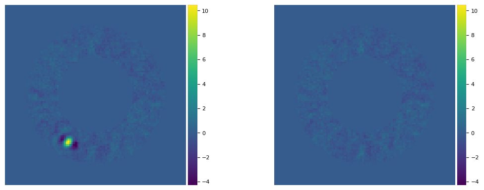
Let’s take a look at the PSF of the planet in the full-frame PCA final image and the same PSF in the frame resulting of processing the planet-subtracted cube:
[23]:
cropped_frame1 = frame_crop(final_ann_opt, cenxy=xy_test, size=15)
New shape: (15, 15)
[24]:
cropped_frame2 = frame_crop(fr_pca_emp, cenxy=xy_test, size=15)
New shape: (15, 15)
Let’s use both 'mode=surface' and the default image mode of plot_frames to show the residuals in the vicinity of the companion:
[25]:
plot_frames((cropped_frame1, cropped_frame2), mode='surface', vmax=8)

[26]:
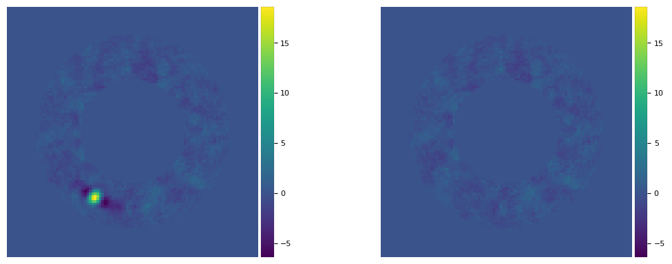
plot_frames((final_ann_opt, fr_pca_emp), vmin = float(np.amin(final_ann_opt)),
            vmax= float(np.amax(final_ann_opt)), axis=False)
Not only the bright point-like signal is subtracted, but so are the negative side lobes. A subtraction not leaving any significant artifact/defect is a good sign that the inferred parameters are correct. However, keep in mind that even for slightly inaccurate parameters, the final image can still look relatively clean. Let’s take for example the parameters inferred with non-optimal \(n_{\rm pc}\):
[27]:
# planet parameters inferred from npc=5 used to make empty cube, then processed with PCA (npc=10)
plpar_fc = [(r_lo[0], theta_lo[0], f_lo[0])]
print(plpar_fc)
cube_emp = cube_planet_free(plpar_fc, cubefc, angs, psfn, imlib=imlib_rot, interpolation=interpolation)
final_ann_5 = pca_annulus(cubefc, angs, ncomp=5, annulus_width=4*fwhm_naco, r_guess=30.5,
                                  imlib=imlib_rot, interpolation=interpolation)
fr_pca_emp5 = pca_annulus(cube_emp, angs, ncomp=5, annulus_width=4*fwhm_naco, r_guess=30.5,
                                  imlib=imlib_rot, interpolation=interpolation)
plot_frames((final_ann_5, fr_pca_emp5), vmin = float(np.amin(final_ann_5)),
            vmax= float(np.amax(final_ann_5)), axis=False)
[(30.534749178951024, 239.97617468137406, 383.05503327816507)]
[28]:
# parameters inferred from npc=25 used to make empty cube, then processed with PCA (npc=10)
plpar_fc = [(r_hi[0], theta_hi[0], f_hi[0])]
print(plpar_fc)
cube_emp = cube_planet_free(plpar_fc, cubefc, angs, psfn, imlib=imlib_rot, interpolation=interpolation)
final_ann_25 = pca_annulus(cubefc, angs, ncomp=25, annulus_width=4*fwhm_naco, r_guess=30.5,
                                   imlib=imlib_rot, interpolation=interpolation)
fr_pca_emp25 = pca_annulus(cube_emp, angs, ncomp=25, annulus_width=4*fwhm_naco, r_guess=30.5,
                                   imlib=imlib_rot, interpolation=interpolation)
plot_frames((final_ann_25, fr_pca_emp25), vmin = float(np.amin(final_ann_25)),
            vmax= float(np.amax(final_ann_25)), axis=False)
[(30.18557073057306, 239.89702835629325, 424.15580033622734)]

Inaccurate parameters still leading to an apparently good removal of the companion brings the question of the uncertainties on each of the three parameters characterizing the companion. The next sections are dedicated to this question.
5.3.3. NEGFC technique coupled with MCMC
5.3.3.1. Running the MCMC sampler
MCMC is a more robust way of obtaining the flux and position. It samples the posterior distributions of the parameters and from them we can infer both the most likely parameter values and uncertainties on each parameter. The relevant function is mcmc_negfc_sampling, which can accept a number of parameters. Let’s define them in the next few boxes:
Let’s first define observation-related parameters, such as the non-coronagraphic psf, its FWHM and the pixel scale od the detector:
[29]:
obs_params = {'psfn': psfn,
              'fwhm': fwhm_naco}
In NEGFC, PCA in a single annulus is used by default to speed up the algorithm - although other algorithms can be used through the algo parameter. Let’s set the \(n_{\rm pc}\) to the optimal \(n_{\rm pc}\) found in Section 5.2. We set the width of the annulus on which PCA is performed (in pixels) with the annulus_width parameter. We also set a few other algorithm-related parameters in the following box:
[30]:
annulus_width = 4*fwhm_naco

algo_params = {'algo': pca_annulus,
               'ncomp': opt_npc_ann,
               'annulus_width': annulus_width,
               'svd_mode': 'lapack',
               'imlib': imlib_rot,
               'interpolation': interpolation}
The choice of log-likelihood expression to be used is determined by mu_sigma and fm. If the former is True (default; mu and sigma calculated automatically) or a tuple of 2 values, the following figure of merit will be used: \(\chi^2 = \sum_j^N \frac{(I_j-\mu)^2}{\sigma^2}\). Otherwise, the choice will be determined by fm: ‘sum’ for the sum of absolute residuals, or ‘stddev’ for the standard deviation of residuals (which can be useful if the point source is contained within a more
extended signal). aperture_radius is the radius of the aperture (in fwhm units) in which the residual intensities \(I_j\) are considered.
[31]:
mu_sigma=True
aperture_radius=2

negfc_params = {'mu_sigma': mu_sigma,
                'aperture_radius': aperture_radius}
Parameter initial_state corresponds to the initial first estimation of the planets parameters (r, theta, flux). We set it to the result of the simplex optimization, obtained with optimal \(n_{\rm pc}\). Note that the MCMC minimization can only run for one companion candidate at a time, hence the first dimension of init should always be 3 (not the number of planets, as opposed to planets_xy_coord in firstguess).
[32]:
initial_state = np.array([r_0[0], theta_0[0], f_0[0]])
Beware that the MCMC procedure is a CPU intensive procedure and can take several hours when run properly on a standard laptop. We use the affine invariant sampler from emcee which can be run in parallel (nproc sets the number of CPUs to be used). At least 100 walkers are recommended for our MCMC chain, although both the number of walkers and iterations will depend on your dataset. For the sake of preventing this tutorial to take too long to run, we set the maximum number of iterations to
500, although feel free to significantly increase it in case of non-convergence.
[33]:
from multiprocessing import cpu_count

nwalkers, itermin, itermax = (100, 200, 500)

mcmc_params = {'nwalkers': nwalkers,
               'niteration_min': itermin,
               'niteration_limit': itermax,
               'bounds': None,
               'nproc': cpu_count()//2}
Another update from Christiaens et al. (2021) is that the convergence can now be evaluated based on the auto-correlation time (see more details in the documentation of ``emcee` <https://emcee.readthedocs.io/en/stable/tutorials/autocorr/>`__), instead of the Gelman-Rubin test, which is inappropriate for non-independent samples (such as an MCMC chain). We set the convergence test to the autocorrelation time based criterion using conv_test='ac' (instead of Gelman-Rubin ‘gb’). We also set the
autocorrelation criterion \(N/\tau >= a_c\), where \(N\) is the number of samples and \(\tau\) the autocorrelation time, to ac_c=50 (the value recommended in the emcee documentation). Finally, we set the number of consecutive times the criterion must be met to: ac_count_thr=1, and the maximum gap in number of steps between 2 checks of the convergence criterion to: check_maxgap=50. If the maximum number of iterations niteration_limit is large enough, the chain will
stop upon meeting the convergence criterion (spoiler: it won’t be the case here since we chose a small value for niteration_limit).
[34]:
conv_test, ac_c, ac_count_thr, check_maxgap = ('ac', 50, 1, 50)

conv_params = {'conv_test': conv_test,
               'ac_c': ac_c,
               'ac_count_thr': ac_count_thr,
               'check_maxgap': check_maxgap}
Setting bounds=None does not mean no bounds are used for parameter exploration, but rather that they are set automatically to:
- \(r \in [r_0-w_{ann}/2, r_0+w_{ann}/2]\), where \(w_{ann}\) is the
annulus_width, - \(\theta \in [\theta_0-\Delta {\rm rot}, \theta_0+\Delta {\rm rot}]\), where \(\Delta {\rm rot}\) is the angle subtended by min(
aperture_radius/2,``fwhm``) at \(r_0\), - \(f \in [0.1*f_0, 2*f_0]\),
where (\(r_0, \theta_0, f_0\)) = initial_state. If the bounds are provided manually (as a tuple of tuples), they will supersede the automatic setting above.
Now let’s start the sampler. Note that this step is computer intensive and may take a long time to run depending on your machine. Feel free to skip the next box if you do not wish to run the MCMC or can’t run it in a reasonable time. The results are already saved as ‘MCMC_results’ in the ‘datasets’ folder and will be loaded in the subsequent boxes.
[35]:
chain = mcmc_negfc_sampling(cubefc, angs, **obs_params, **algo_params, **negfc_params,
                            initial_state=initial_state, **mcmc_params, **conv_params,
                            display=True, verbosity=2, save=False, output_dir='./')
――――――――――――――――――――――――――――――――――――――――――――――――――――――――――――――――――――――――――――――――
Starting time: 2022-05-04 13:39:04
――――――――――――――――――――――――――――――――――――――――――――――――――――――――――――――――――――――――――――――――
        MCMC sampler for the NEGFC technique
――――――――――――――――――――――――――――――――――――――――――――――――――――――――――――――――――――――――――――――――
The mean and stddev in the annulus at the radius of the companion (excluding the PA area directly adjacent to it) are -0.01 and 1.48 respectively.
Beginning emcee Ensemble sampler...
emcee Ensemble sampler successful

Start of the MCMC run ...
Step  |  Duration/step (sec)  |  Remaining Estimated Time (sec)
0               3.47851                 1735.77874
1               1.38965                 692.04520
2               1.38548                 688.58207
3               1.36664                 677.85542
4               1.37508                 680.66460
5               1.38777                 685.55739
6               1.36152                 671.22936
7               1.37935                 678.63823
8               1.39976                 687.28216
9               1.38258                 677.46469
10              1.36537                 667.66397
11              1.37168                 669.37935
12              1.36878                 666.59781
13              1.36647                 664.10636
14              1.36966                 664.28704
15              1.36997                 663.06451
16              1.36980                 661.61340
17              1.38879                 669.39823
18              1.37246                 660.15182
19              1.38434                 664.48368
20              1.37649                 659.34063
21              1.36439                 652.18033
22              1.36600                 651.58152
23              1.36397                 649.24734
24              1.36953                 650.52723
25              1.36554                 647.26454
26              1.37040                 648.19873
27              1.36910                 646.21567
28              1.36674                 643.73219
29              1.37244                 645.04821
30              1.36953                 642.31191
31              1.37786                 644.83801
32              1.36838                 639.03486
33              1.37587                 641.15728
34              1.38366                 643.40190
35              1.37418                 637.61859
36              1.36562                 632.28345
37              1.37518                 635.33316
38              1.37097                 632.01717
39              1.37377                 631.93512
40              1.36616                 627.06744
41              1.41404                 647.63032
42              1.42133                 649.54918
43              1.37764                 628.20202
44              1.37153                 624.04660
45              1.38171                 627.29725
46              1.37053                 620.85100
47              1.37285                 620.52639
48              1.36444                 615.36064
49              1.36433                 613.94895
50              1.36821                 614.32449

 ac convergence test in progress...
51              1.75774                 787.46618
52              1.37224                 613.39083
53              1.36716                 609.75158
54              1.36701                 608.31945
55              1.37034                 608.42963
56              1.36799                 606.01824
57              1.36227                 602.12511
58              1.37602                 606.82438
59              1.37225                 603.79000
60              1.36685                 600.04496
61              1.36519                 597.95497
62              1.35685                 592.94476
63              1.36890                 596.84084
64              1.36670                 594.51493
65              1.37584                 597.11499
66              1.36403                 590.62542
67              1.36657                 590.35824
68              1.36726                 589.28906
69              1.36786                 588.18109
70              1.35679                 582.06377
71              1.36564                 584.49349
72              1.36407                 582.45618
73              1.36285                 580.57410
74              1.35704                 576.74115
75              1.36997                 580.86940
76              1.38369                 585.30214
77              1.38872                 586.03984
78              1.39496                 587.27816
79              1.39433                 585.61944
80              1.38035                 578.36749
81              1.39219                 581.93542
82              1.37591                 573.75447
83              1.37403                 571.59440
84              1.37887                 572.22897
85              1.46772                 607.63442
86              1.38292                 571.14761
87              1.36528                 562.49618
88              1.36131                 559.49800
89              1.37875                 565.28586
90              1.37170                 561.02407
91              1.36405                 556.53118
92              1.37014                 557.64495
93              1.36063                 552.41416
94              1.36496                 552.80799
95              1.35604                 547.83895
96              1.37475                 554.02224
97              1.35842                 546.08323
98              1.36179                 546.07699
99              1.37333                 549.33040
100             1.38278                 551.73002

 ac convergence test in progress...
101             1.93721                 771.00878
102             1.36099                 540.31224
103             1.37314                 543.76502
104             1.36566                 539.43491
105             1.37684                 542.47299
106             1.39130                 546.78090
107             1.37662                 539.63347
108             1.37140                 536.21896
109             1.36952                 534.11124
110             1.36918                 532.61063
111             1.36899                 531.16967
112             1.35915                 525.98911
113             1.35839                 524.33700
114             1.36695                 526.27498
115             1.36556                 524.37466
116             1.36960                 524.55527
117             1.37089                 523.68189
118             1.35611                 516.67677
119             1.37855                 523.85014
120             1.37659                 521.72723
121             1.35964                 513.94316
122             1.36840                 515.88793
123             1.37461                 516.85336
124             1.36725                 512.71837
125             1.36842                 511.78833
126             1.35909                 506.94020
127             1.36349                 507.21642
128             1.40657                 521.83858
129             1.39825                 517.35398
130             1.37142                 506.05361
131             1.36641                 502.83778
132             1.35998                 499.11303
133             1.37224                 502.23984
134             1.36263                 497.36031
135             1.36428                 496.59646
136             1.38187                 501.61881
137             1.35364                 490.01804
138             1.35730                 489.98602
139             1.37474                 494.90640
140             1.36030                 488.34770
141             1.36739                 489.52383
142             1.36742                 488.16894
143             1.37003                 487.73175
144             1.37192                 487.03195
145             1.35985                 481.38584
146             1.35557                 478.51797
147             1.36797                 481.52685
148             1.36882                 480.45547
149             1.36526                 477.84205
150             1.38094                 481.94876

 ac convergence test in progress...

151             1.75770                 611.67786
152             1.36334                 473.07933
153             1.36924                 473.75739
154             1.36606                 471.29104
155             1.36057                 468.03608
156             1.37101                 470.25540
157             1.36387                 466.44491
158             1.36719                 466.21077
159             1.36894                 465.43858
160             1.36576                 462.99366
161             1.36094                 459.99907
162             1.36516                 460.05926
163             1.37645                 462.48821
164             1.37219                 459.68466
165             1.35647                 453.06031
166             1.36374                 454.12475
167             1.35243                 449.00610
168             1.37150                 453.96617
169             1.37865                 454.95516
170             1.37030                 450.82771
171             1.39785                 458.49513
172             1.43137                 468.05701
173             1.37182                 447.21299
174             1.36833                 444.70757
175             1.35695                 439.65245
176             1.37037                 442.62854
177             1.36034                 438.02819
178             1.36000                 436.56000
179             1.36537                 436.91840
180             1.37311                 438.02337
181             1.36582                 434.33012
182             1.37269                 435.14368
183             1.36729                 432.06490
184             1.36564                 430.17597
185             1.37111                 430.52854
186             1.34831                 422.02259
187             1.35744                 423.52128
188             1.39528                 433.93332
189             1.36377                 422.76808
190             1.36072                 420.46186
191             1.35898                 418.56522
192             1.36317                 418.49411
193             1.38411                 423.53888
194             1.36445                 416.15786
195             1.35518                 411.97320
196             1.37015                 415.15515
197             1.36743                 412.96537
198             1.35415                 407.60005
199             1.35116                 405.34650
200             1.35808                 406.06562

 ac convergence test in progress...
Auto-corr tau/N = [0.06893561 0.06749297 0.0631891 ]
tau/N <= 0.02 = [False False False]

201             1.77288                 528.31913
202             1.37000                 406.88881
203             1.37306                 406.42458
204             1.36606                 402.98711
205             1.36417                 401.06569
206             1.36871                 401.03203
207             1.37946                 402.80320
208             1.36279                 396.57131
209             1.36843                 396.84499
210             1.37597                 397.65446
211             1.36622                 393.47050
212             1.36528                 391.83536
213             1.36224                 389.60121
214             1.36528                 389.10395
215             1.43257                 406.84931
216             1.43605                 406.40187
217             1.36902                 386.06279
218             1.36523                 383.62935
219             1.35951                 380.66364
220             1.37400                 383.34656
221             1.35613                 377.00386
222             1.36476                 378.03907
223             1.35997                 375.35282
224             1.37137                 377.12757
225             1.35623                 371.60757
226             1.36196                 371.81617
227             1.36167                 370.37560
228             1.36531                 369.99955
229             1.37026                 369.97047
230             1.36312                 366.67794
231             1.35774                 363.87432
232             1.36135                 363.48045
233             1.36352                 362.69499
234             1.36618                 362.03664
235             1.36623                 360.68393
236             1.36985                 360.27055
237             1.37298                 359.72024
238             1.36663                 356.69147
239             1.36002                 353.60442
240             1.36172                 352.68626
241             1.36940                 353.30546
242             1.37169                 352.52356
243             1.37288                 351.45856
244             1.36466                 347.98932
245             1.36358                 346.34907
246             1.36706                 345.86643
247             1.36993                 345.22160
248             1.37215                 344.40890
249             1.36566                 341.41525
250             1.36199                 339.13501

 ac convergence test in progress...
Auto-corr tau/N = [0.06364067 0.06439249 0.06246105]
tau/N <= 0.02 = [False False False]

251             1.94756                 482.99538
252             1.36337                 336.75140
253             1.36100                 334.80649
254             1.37141                 335.99520
255             1.37027                 334.34564
256             1.37115                 333.18945
257             1.36799                 331.05406
258             1.44828                 349.03452
259             1.44380                 346.51224
260             1.36711                 326.74001
261             1.37324                 326.83041
262             1.36312                 323.06062
263             1.36307                 321.68428
264             1.37064                 322.10087
265             1.35906                 318.01910
266             1.36530                 318.11467
267             1.36447                 316.55727
268             1.36189                 314.59728
269             1.38437                 318.40625
270             1.36441                 312.45081
271             1.35902                 309.85565
272             1.37468                 312.05191
273             1.36083                 307.54781
274             1.36878                 307.97482
275             1.36476                 305.70714
276             1.35680                 302.56662
277             1.36779                 303.64938
278             1.37177                 303.16051
279             1.36021                 299.24664
280             1.36642                 299.24598
281             1.36069                 296.62977
282             1.36457                 296.11256
283             1.36525                 294.89378
284             1.36005                 292.41139
285             1.36183                 291.43141
286             1.36830                 291.44747
287             1.36051                 288.42770
288             1.36444                 287.89768
289             1.36100                 285.81084
290             1.36291                 284.84882
291             1.36013                 282.90787
292             1.36963                 283.51403
293             1.36475                 281.13891
294             1.35840                 278.47262
295             1.36955                 279.38881
296             1.37323                 278.76630
297             1.36603                 275.93766
298             1.36052                 273.46392
299             1.35451                 270.90260
300             1.37308                 273.24232

 ac convergence test in progress...
Auto-corr tau/N = [0.05879776 0.05591288 0.06160337]
tau/N <= 0.02 = [False False False]

301             1.80238                 356.87124
302             1.44800                 285.25659
303             1.42286                 278.88036
304             1.36092                 265.37999
305             1.35983                 263.80624
306             1.36730                 263.88967
307             1.36941                 262.92595
308             1.36853                 261.38866
309             1.36217                 258.81325
310             1.36594                 258.16190
311             1.37018                 257.59403
312             1.36369                 255.01003
313             1.36981                 254.78429
314             1.35805                 251.23907
315             1.35745                 249.77154
316             1.38237                 252.97298
317             1.38293                 251.69253
318             1.37136                 248.21598
319             1.36390                 245.50290
320             1.36443                 244.23351
321             1.37658                 245.03053
322             1.36869                 242.25902
323             1.37047                 241.20202
324             1.35917                 237.85405
325             1.36901                 238.20739
326             1.37334                 237.58799
327             1.37183                 235.95562
328             1.35928                 232.43603
329             1.37152                 233.15823
330             1.36776                 231.15212
331             1.37223                 230.53414
332             1.35824                 226.82541
333             1.37457                 228.17912
334             1.36473                 225.18095
335             1.37727                 225.87244
336             1.36999                 223.30756
337             1.36504                 221.13599
338             1.37452                 221.29740
339             1.37399                 219.83856
340             1.36184                 216.53256
341             1.37440                 217.15473
342             1.35969                 213.47180
343             1.36336                 212.68369
344             1.36208                 211.12256
345             1.36396                 210.04969
346             1.48087                 226.57342
347             1.36201                 207.02537
348             1.32350                 199.84850
349             1.34267                 201.39990
350             1.32945                 198.08850

 ac convergence test in progress...
Auto-corr tau/N = [0.05431862 0.05251512 0.05584251]
tau/N <= 0.02 = [False False False]

351             1.75272                 259.40256
352             1.34394                 197.55977
353             1.34163                 195.87856
354             1.34003                 194.30435
355             1.34685                 193.94611
356             1.32480                 189.44626
357             1.32372                 187.96796
358             1.32240                 186.45812
359             1.32098                 184.93706
360             1.34424                 186.84964
361             1.32233                 182.48195
362             1.34912                 184.82930
363             1.32204                 179.79717
364             1.32098                 178.33216
365             1.33035                 178.26690
366             1.36083                 180.99052
367             1.38104                 182.29702
368             1.35296                 177.23815
369             1.35963                 176.75164
370             1.32232                 170.57876
371             1.32080                 169.06291
372             1.31747                 167.31907
373             1.34191                 169.08079
374             1.32056                 165.07025
375             1.34571                 166.86779
376             1.35669                 166.87336
377             1.35366                 165.14664
378             1.32598                 160.44370
379             1.32274                 158.72928
380             1.32460                 157.62764
381             1.36931                 161.57905
382             1.32920                 155.51640
383             1.32964                 154.23789
384             1.35979                 156.37608
385             1.36325                 155.41004
386             1.32564                 149.79777
387             1.32717                 148.64326
388             1.35921                 150.87242
389             1.35952                 149.54687
390             1.42843                 155.69843
391             1.45226                 156.84397
392             1.32920                 142.22472
393             1.32644                 140.60243
394             1.34765                 141.50357
395             1.33825                 139.17758
396             1.32440                 136.41351
397             1.33204                 135.86839
398             1.33378                 134.71218
399             1.33044                 133.04370
400             1.32203                 130.88137

 ac convergence test in progress...

Auto-corr tau/N = [0.05007131 0.04780584 0.04992041]
tau/N <= 0.02 = [False False False]

401             1.94558                 190.66704
402             1.35482                 131.41773
403             1.34879                 129.48432
404             1.33167                 126.50894
405             1.33250                 125.25491
406             1.32852                 123.55255
407             1.32884                 122.25346
408             1.33683                 121.65144
409             1.32430                 119.18727
410             1.34801                 119.97316
411             1.32566                 116.65764
412             1.32543                 115.31224
413             1.32671                 114.09740
414             1.35313                 115.01605
415             1.37420                 115.43297
416             1.36264                 113.09895
417             1.35015                 110.71214
418             1.32385                 107.23169
419             1.32301                 105.84048
420             1.35332                 106.91267
421             1.31920                 102.89776
422             1.34429                 103.51025
423             1.35127                 102.69629
424             1.32177                 99.13260
425             1.32626                 98.14294
426             1.33582                 97.51493
427             1.32242                 95.21410
428             1.32658                 94.18725
429             1.33272                 93.29040
430             1.31968                 91.05820
431             1.32835                 90.32746
432             1.37294                 91.98664
433             1.32567                 87.49415
434             1.39452                 90.64354
435             1.42596                 91.26157
436             1.33659                 84.20511
437             1.35165                 83.80242
438             1.34022                 81.75366
439             1.34367                 80.62038
440             1.33631                 78.84241
441             1.35414                 78.54024
442             1.33743                 76.23368
443             1.34242                 75.17546
444             1.34213                 73.81715
445             1.35488                 73.16330
446             1.34346                 71.20317
447             1.33739                 69.54444
448             1.33476                 68.07291
449             1.35572                 67.78575
450             1.33413                 65.37247

 ac convergence test in progress...
Auto-corr tau/N = [0.0461422  0.04651919 0.04701059]
tau/N <= 0.02 = [False False False]

451             1.78397                 85.63051
452             1.34145                 63.04829
453             1.33849                 61.57077
454             1.34721                 60.62454
455             1.34479                 59.17063
456             1.37163                 58.98030
457             1.35656                 56.97544
458             1.34790                 55.26402
459             1.33506                 53.40248
460             1.33735                 52.15646
461             1.31649                 50.02654
462             1.33691                 49.46552
463             1.32977                 47.87183
464             1.36603                 47.81091
465             1.34201                 45.62824
466             1.34397                 44.35098
467             1.34131                 42.92189
468             1.36327                 42.26140
469             1.33844                 40.15329
470             1.34606                 39.03560
471             1.34264                 37.59400
472             1.35083                 36.47246
473             1.34537                 34.97962
474             1.36461                 34.11512
475             1.35284                 32.46811
476             1.33381                 30.67763
477             1.33902                 29.45851
478             1.40367                 29.47703
479             1.47148                 29.42952
480             1.38129                 26.24453
481             1.35009                 24.30162
482             1.34242                 22.82122
483             1.34057                 21.44912
484             1.34618                 20.19270
485             1.35671                 18.99397
486             1.35507                 17.61594
487             1.33743                 16.04915
488             1.35180                 14.86977
489             1.34272                 13.42715
490             1.37927                 12.41345
491             1.34466                 10.75728
492             1.35501                 9.48506
493             1.33119                 7.98712
494             1.34971                 6.74856
495             1.34203                 5.36812
496             1.35477                 4.06430
497             1.33913                 2.67826
498             1.33900                 1.33900
499             1.34192                 0.00000
We have reached the limit # of steps without convergence
Running time:  0:11:31.680492
――――――――――――――――――――――――――――――――――――――――――――――――――――――――――――――――――――――――――――――――
If you ran the previous box and wish to write your results, set write=True in the next box. This will pickle the MCMC chain.
[36]:
write=False

if write:
    import pickle
    output = {'chain':chain}
    with open('../datasets/my_MCMC_results', 'wb') as fileSave:
        pickle.dump(output, fileSave)
Note that an alternative to the box above, is to provide output_dir in the call to mcmc_negfc_sampling and set save to True. This will save the results as a pickle including additional keys: apart from ‘chain’, it will also save ‘input_parameters’, ‘AR’ (acceptance ratio), and ‘lnprobability’.
Pickled results can be loaded from disk like this:
[37]:
import pickle
with open('../datasets/MCMC_results','rb') as fi:
    myPickler = pickle.Unpickler(fi)
    mcmc_result = myPickler.load()

print(mcmc_result.keys())
chain = mcmc_result['chain']
dict_keys(['chain', 'input_parameters', 'AR', 'lnprobability'])
The most accurate approach would involve setting a large enough maximum number of iterations and using FFT-based rotation for PCA. The latter in particular, may change a bit the most likely parameter values given the better flux conservation. However, these changes would involve over ~3 orders of magnitude longer calculation time. It is therefore intractable for a personal laptop and not shown in this notebook. If you have access to a supercomputer feel free to adopt these changes though. The results after 500 iterations are nonetheless good enough for illustrative purpose:
5.3.3.2. Visualizing the MCMC chain: corner plots and walk plots
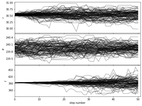
Let’s first check that the walk plots look ok:
[38]:
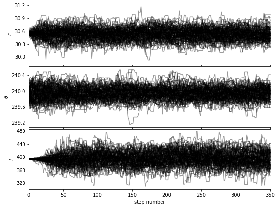
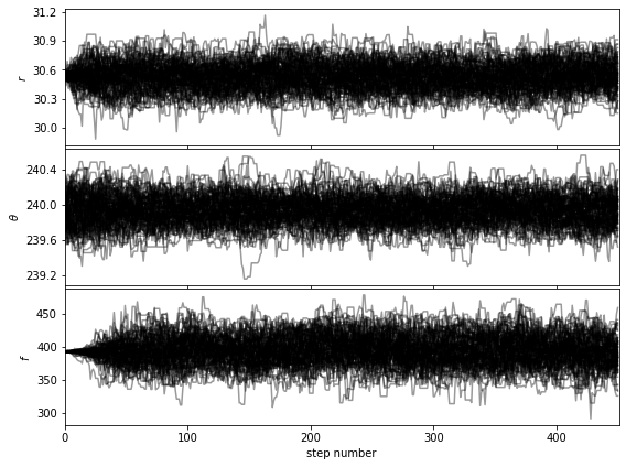
show_walk_plot(chain)
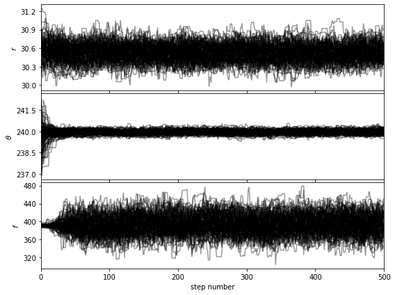
Then based on the walk plot, let’s burn-in the first 30% of the chain, to calculate the corner plots:
[39]:
burnin = 0.3
burned_chain = chain[:, int(chain.shape[1]//(1/burnin)):, :]
show_corner_plot(burned_chain)

For the purpose of this tutorial and to limit computation time we set the maximum number of iterations to 500 for 100 walkers. The look of the corner plots may improve with more samples (i.e. higher number of iterations, for a given burn-in ratio). This can be tested by setting the max. number of iterations arbitrarily high for the autocorrelation-time convergence criterion to be met.
5.3.3.3. Highly probable values and confidence intervals
Now let’s determine the most highly probable value for each model parameter, as well as the 1-sigma confidence interval. For this, let’s first flatten the chains:
[40]:
isamples_flat = chain[:, int(chain.shape[1]//(1/burnin)):, :].reshape((-1,3))
Then use the confidence function:
[41]:
val_max, conf = confidence(isamples_flat, cfd=68, gaussian_fit=False, verbose=True, save=False,
                           gt=gt, ndig=1, title=True)
percentage for r: 69.79202279202278%
percentage for theta: 69.02279202279202%
percentage for f: 68.94017094017094%


Confidence intervals:
r: 30.57489764243517 [-0.20421878422770945,0.08279139901123145]
theta: 239.91771004343246 [-0.14527599962792692,0.18317408648738365]
f: 390.7650582608513 [-20.054061636888093,25.285555976945886]
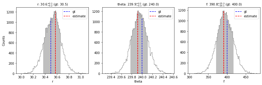
Using the confidence function with the gaussian_fit=True option, it is possible to fit a Gaussian to the posterior distribution of each parameter, and infer associated uncertainty values.
[42]:
mu, sigma = confidence(isamples_flat, cfd=68, gaussian_fit=True, verbose=True, save=False,
                       gt=gt, ndig=1, title=True)
percentage for r: 69.79202279202278%
percentage for theta: 69.02279202279202%
percentage for f: 68.94017094017094%


Confidence intervals:
r: 30.57489764243517 [-0.20421878422770945,0.08279139901123145]
theta: 239.91771004343246 [-0.14527599962792692,0.18317408648738365]
f: 390.7650582608513 [-20.054061636888093,25.285555976945886]

Gaussian fit results:
r: 30.525747462344565 +-0.13676103149725966
theta: 239.94793373875024 +-0.15744912409220196
f: 394.1338634773366 +-21.669634439677626

It is recommended to report the results as confidence intervals (i.e. with possibly asymmetric uncertainties) as long as the bin interval is small enough. Here, we also fitted the residual posterior distribution of each parameter to a Gaussian distribution (this shape is the expected one if the noise has been well whitened, but is not necessarily guaranteed at all separations depending on the adopted \(n_{\rm pc}\)). In case, these distributions look Gaussian, the inferred \(\sigma\) value may be a more accurate uncertainty value for the different parameters.
We can see that the confidence intervals inferred by NEGFC for the different parameters encompass the ground truth values used for injection (in particular for the flux).
Note that depending on your choice of mu_sigma, you may have to calculate separately another source of uncertainty. Indeed, with the original expression for \(\chi^2\) (Wertz et al. 2017; mu_sigma=False), only the uncertainty associated to photon noise was reflected in the MCMC results. With the new expression (mu_sigma=True), the \(\chi^2\) expression also takes into account the residual speckle noise at the radial separation of the companion candidate. Our tests suggest
that similar final uncertainties can be obtained in either of these 2 ways:
- the uncertainties obtained with MCMC when setting
mu_sigma=True; - the uncertainties obtained by combining quadratically the uncertainties obtained with MCMC (setting
mu_sigma=Falseandfm = 'sum'), and the residual speckle uncertainties inferred as in Sec. 5.3.4 (Wertz et al. 2017).
5.3.4. Residual speckle uncertainty
Only needed if using ``mu_sigma=False`` in your call to mcmc_negfc_sampling!
Residual speckle noise can also bias the best parameter estimates found for the companion (if not taken into account in the MCMC). To evaluate the uncertainty associated to this additional source of noise, it is recommended to inject a large number of fake companions at the same radius and flux as estimated for the true companion but different azimuths, and then estimate their parameters using simplex-NEGFC. The distribution of differences with respect to injected parameters can then give us an
idea of the residual speckle noise uncertainty. This is done in VIP with the speckle_noise_uncertainty function (see also Sec. 3.3 in Wertz et al. 2017 for more details).
Let’s use the planet parameters inferred by the MCMC-NEGFC algorithm:
[43]:
pl_par = (val_max['r'],val_max['theta'],val_max['f'])
pl_par
[43]:
(30.57489764243517, 239.91771004343246, 390.7650582608513)
[44]:
algo_options={'ncomp':opt_npc_ann, 'annulus_width':4*fwhm_naco, 'imlib':imlib_rot,
              'interpolation':interpolation}
speckle_res = speckle_noise_uncertainty(cubefc, pl_par, np.linspace(0,359,360), angs, pca_annulus,
                                        psfn, fwhm_naco, aperture_radius=2, fmerit='sum',
                                        algo_options=algo_options, transmission=None, mu_sigma=None,
                                        wedge=None, weights=None, force_rPA=False, nproc=None,
                                        simplex_options=None, bins=None, save=False, output=None,
                                        verbose=True, full_output=True, plot=True)
#######################################################
###            SPECKLE NOISE DETERMINATION          ###
#######################################################

Number of steps: 360

Process is running for angle: 0.00
Process is running for angle: 18.00
Process is running for angle: 36.00
Process is running for angle: 54.00
Process is running for angle: 72.00
Process is running for angle: 1.00
Process is running for angle: 37.00
Process is running for angle: 19.00
Process is running for angle: 73.00
Process is running for angle: 55.00
Process is running for angle: 38.00
Process is running for angle: 2.00
Process is running for angle: 20.00
Process is running for angle: 74.00
Process is running for angle: 56.00
Process is running for angle: 39.00
Process is running for angle: 3.00
Process is running for angle: 75.00
Process is running for angle: 21.00
Process is running for angle: 40.00
Process is running for angle: 57.00
Process is running for angle: 4.00
Process is running for angle: 76.00
Process is running for angle: 22.00
Process is running for angle: 41.00
Process is running for angle: 58.00
Process is running for angle: 23.00
Process is running for angle: 5.00
Process is running for angle: 77.00
Process is running for angle: 42.00
Process is running for angle: 24.00
Process is running for angle: 59.00
Process is running for angle: 6.00
Process is running for angle: 78.00
Process is running for angle: 43.00
Process is running for angle: 25.00
Process is running for angle: 60.00
Process is running for angle: 7.00
Process is running for angle: 79.00
Process is running for angle: 26.00
Process is running for angle: 8.00
Process is running for angle: 61.00
Process is running for angle: 44.00
Process is running for angle: 27.00
Process is running for angle: 45.00
Process is running for angle: 62.00
Process is running for angle: 9.00
Process is running for angle: 80.00
Process is running for angle: 28.00
Process is running for angle: 63.00
Process is running for angle: 46.00
Process is running for angle: 10.00
Process is running for angle: 81.00
Process is running for angle: 29.00
Process is running for angle: 64.00
Process is running for angle: 47.00
Process is running for angle: 11.00
Process is running for angle: 82.00
Process is running for angle: 30.00
Process is running for angle: 65.00
Process is running for angle: 48.00
Process is running for angle: 12.00
Process is running for angle: 31.00
Process is running for angle: 83.00
Process is running for angle: 66.00
Process is running for angle: 49.00
Process is running for angle: 13.00
Process is running for angle: 32.00
Process is running for angle: 67.00
Process is running for angle: 14.00
Process is running for angle: 84.00
Process is running for angle: 50.00
Process is running for angle: 33.00
Process is running for angle: 15.00
Process is running for angle: 68.00
Process is running for angle: 85.00
Process is running for angle: 51.00
Process is running for angle: 16.00
Process is running for angle: 34.00
Process is running for angle: 69.00
Process is running for angle: 86.00
Process is running for angle: 52.00
Process is running for angle: 35.00
Process is running for angle: 17.00
Process is running for angle: 70.00
Process is running for angle: 87.00
Process is running for angle: 90.00
Process is running for angle: 53.00
Process is running for angle: 108.00
Process is running for angle: 88.00
Process is running for angle: 71.00
Process is running for angle: 126.00
Process is running for angle: 109.00
Process is running for angle: 91.00
Process is running for angle: 89.00
Process is running for angle: 127.00
Process is running for angle: 144.00
Process is running for angle: 110.00
Process is running for angle: 162.00
Process is running for angle: 92.00
Process is running for angle: 128.00
Process is running for angle: 145.00
Process is running for angle: 111.00
Process is running for angle: 93.00
Process is running for angle: 163.00
Process is running for angle: 129.00
Process is running for angle: 112.00
Process is running for angle: 94.00
Process is running for angle: 164.00
Process is running for angle: 146.00
Process is running for angle: 130.00
Process is running for angle: 113.00
Process is running for angle: 147.00
Process is running for angle: 165.00
Process is running for angle: 95.00
Process is running for angle: 131.00
Process is running for angle: 148.00
Process is running for angle: 114.00
Process is running for angle: 96.00
Process is running for angle: 166.00
Process is running for angle: 132.00
Process is running for angle: 149.00
Process is running for angle: 115.00
Process is running for angle: 167.00
Process is running for angle: 97.00
Process is running for angle: 133.00
Process is running for angle: 150.00
Process is running for angle: 98.00
Process is running for angle: 116.00
Process is running for angle: 134.00
Process is running for angle: 168.00
Process is running for angle: 151.00
Process is running for angle: 135.00
Process is running for angle: 117.00
Process is running for angle: 99.00
Process is running for angle: 169.00
Process is running for angle: 152.00
Process is running for angle: 136.00
Process is running for angle: 100.00
Process is running for angle: 118.00
Process is running for angle: 170.00
Process is running for angle: 137.00
Process is running for angle: 153.00
Process is running for angle: 101.00
Process is running for angle: 119.00
Process is running for angle: 171.00
Process is running for angle: 154.00
Process is running for angle: 138.00
Process is running for angle: 102.00
Process is running for angle: 120.00
Process is running for angle: 155.00
Process is running for angle: 139.00
Process is running for angle: 172.00
Process is running for angle: 103.00
Process is running for angle: 121.00
Process is running for angle: 140.00
Process is running for angle: 156.00
Process is running for angle: 173.00
Process is running for angle: 104.00
Process is running for angle: 141.00
Process is running for angle: 122.00
Process is running for angle: 157.00
Process is running for angle: 174.00
Process is running for angle: 142.00
Process is running for angle: 158.00
Process is running for angle: 105.00
Process is running for angle: 123.00
Process is running for angle: 175.00
Process is running for angle: 159.00
Process is running for angle: 124.00
Process is running for angle: 106.00
Process is running for angle: 143.00
Process is running for angle: 125.00
Process is running for angle: 180.00
Process is running for angle: 176.00
Process is running for angle: 107.00
Process is running for angle: 160.00
Process is running for angle: 198.00
Process is running for angle: 181.00
Process is running for angle: 177.00
Process is running for angle: 161.00
Process is running for angle: 216.00
Process is running for angle: 178.00
Process is running for angle: 199.00
Process is running for angle: 182.00
Process is running for angle: 234.00
Process is running for angle: 217.00
Process is running for angle: 179.00
Process is running for angle: 183.00
Process is running for angle: 200.00
Process is running for angle: 235.00
Process is running for angle: 252.00
Process is running for angle: 218.00
Process is running for angle: 236.00
Process is running for angle: 184.00
Process is running for angle: 201.00
Process is running for angle: 253.00
Process is running for angle: 219.00
Process is running for angle: 185.00
Process is running for angle: 237.00
Process is running for angle: 254.00
Process is running for angle: 202.00
Process is running for angle: 186.00
Process is running for angle: 238.00
Process is running for angle: 220.00
Process is running for angle: 203.00
Process is running for angle: 255.00
Process is running for angle: 239.00
Process is running for angle: 187.00
Process is running for angle: 256.00
Process is running for angle: 240.00
Process is running for angle: 221.00
Process is running for angle: 188.00
Process is running for angle: 204.00
Process is running for angle: 257.00
Process is running for angle: 241.00
Process is running for angle: 189.00
Process is running for angle: 205.00
Process is running for angle: 222.00
Process is running for angle: 258.00
Process is running for angle: 190.00
Process is running for angle: 242.00
Process is running for angle: 223.00
Process is running for angle: 206.00
Process is running for angle: 259.00
Process is running for angle: 191.00
Process is running for angle: 224.00
Process is running for angle: 207.00
Process is running for angle: 243.00
Process is running for angle: 260.00
Process is running for angle: 225.00
Process is running for angle: 244.00
Process is running for angle: 208.00
Process is running for angle: 261.00
Process is running for angle: 192.00
Process is running for angle: 245.00
Process is running for angle: 209.00
Process is running for angle: 193.00
Process is running for angle: 226.00
Process is running for angle: 262.00
Process is running for angle: 246.00
Process is running for angle: 210.00
Process is running for angle: 194.00
Process is running for angle: 227.00
Process is running for angle: 263.00
Process is running for angle: 247.00
Process is running for angle: 211.00
Process is running for angle: 264.00
Process is running for angle: 195.00
Process is running for angle: 228.00
Process is running for angle: 248.00
Process is running for angle: 265.00
Process is running for angle: 212.00
Process is running for angle: 229.00
Process is running for angle: 196.00
Process is running for angle: 249.00
Process is running for angle: 266.00
Process is running for angle: 230.00
Process is running for angle: 197.00
Process is running for angle: 213.00
Process is running for angle: 250.00
Process is running for angle: 267.00
Process is running for angle: 231.00
Process is running for angle: 214.00
Process is running for angle: 251.00
Process is running for angle: 270.00
Process is running for angle: 268.00
Process is running for angle: 232.00
Process is running for angle: 288.00
Process is running for angle: 215.00
Process is running for angle: 271.00
Process is running for angle: 289.00
Process is running for angle: 233.00
Process is running for angle: 272.00
Process is running for angle: 269.00
Process is running for angle: 306.00
Process is running for angle: 290.00
Process is running for angle: 324.00
Process is running for angle: 273.00
Process is running for angle: 307.00
Process is running for angle: 342.00
Process is running for angle: 325.00
Process is running for angle: 291.00
Process is running for angle: 308.00
Process is running for angle: 274.00
Process is running for angle: 343.00
Process is running for angle: 326.00
Process is running for angle: 275.00
Process is running for angle: 309.00
Process is running for angle: 344.00
Process is running for angle: 292.00
Process is running for angle: 327.00
Process is running for angle: 310.00
Process is running for angle: 276.00
Process is running for angle: 345.00
Process is running for angle: 328.00
Process is running for angle: 293.00
Process is running for angle: 311.00
Process is running for angle: 277.00
Process is running for angle: 346.00
Process is running for angle: 294.00
Process is running for angle: 312.00
Process is running for angle: 329.00
Process is running for angle: 278.00
Process is running for angle: 295.00
Process is running for angle: 347.00
Process is running for angle: 313.00
Process is running for angle: 279.00
Process is running for angle: 330.00
Process is running for angle: 348.00
Process is running for angle: 280.00
Process is running for angle: 296.00
Process is running for angle: 331.00
Process is running for angle: 314.00
Process is running for angle: 349.00
Process is running for angle: 281.00
Process is running for angle: 332.00
Process is running for angle: 315.00
Process is running for angle: 297.00
Process is running for angle: 282.00
Process is running for angle: 333.00
Process is running for angle: 316.00
Process is running for angle: 350.00
Process is running for angle: 298.00
Process is running for angle: 334.00
Process is running for angle: 283.00
Process is running for angle: 317.00
Process is running for angle: 351.00
Process is running for angle: 335.00
Process is running for angle: 299.00
Process is running for angle: 284.00
Process is running for angle: 318.00
Process is running for angle: 336.00
Process is running for angle: 285.00
Process is running for angle: 352.00
Process is running for angle: 300.00
Process is running for angle: 337.00
Process is running for angle: 319.00
Process is running for angle: 286.00
Process is running for angle: 353.00
Process is running for angle: 301.00
Process is running for angle: 338.00
Process is running for angle: 320.00
Process is running for angle: 287.00
Process is running for angle: 354.00
Process is running for angle: 321.00
Process is running for angle: 339.00
Process is running for angle: 302.00
Process is running for angle: 355.00
Process is running for angle: 322.00
Process is running for angle: 340.00
Process is running for angle: 323.00
Process is running for angle: 303.00
Process is running for angle: 356.00
Process is running for angle: 341.00
Process is running for angle: 304.00
Process is running for angle: 357.00
Process is running for angle: 305.00
Process is running for angle: 358.00
Process is running for angle: 359.00
residuals (offsets):  [ 0.01415679  0.02621993 -0.02744315  0.00635802  0.00837833 -0.0176962
 -0.03312964 -0.0547925  -0.06124026 -0.07192343 -0.06382566 -0.07711383
 -0.09335087 -0.06946001 -0.02784876 -0.01598752  0.02652482  0.0526809
  0.10291377  0.07627605  0.08016999  0.12327355  0.04013548 -0.01765467
 -0.05793429 -0.08913544 -0.07950251 -0.14093212 -0.1179294  -0.11975682
 -0.10624286 -0.09006137 -0.08172908 -0.010413   -0.00552254  0.00274251
  0.04476128  0.01594012  0.02296539  0.01412726  0.01801435 -0.01715912
 -0.01237452  0.0053138  -0.01071325  0.03306639  0.03159408  0.07173099
  0.05520899  0.05662432  0.06153248  0.04479955  0.0446696   0.05382092
  0.04781707  0.042598    0.02748159 -0.0064816  -0.02805345 -0.0473227
 -0.08893345 -0.08833836 -0.08534747 -0.07996837 -0.09014496 -0.03539202
 -0.0025495   0.01278922  0.00407768  0.00029818  0.03154075  0.01252282
  0.01683253  0.0227989  -0.00583583  0.01100947  0.01884958  0.01248943
  0.01915697 -0.05120149 -0.02140614 -0.03594936 -0.01526049 -0.03755925
  0.0020905  -0.01593293  0.02130371  0.070312    0.05976488 -0.10668152
 -0.00836779 -0.11304176 -0.10291612 -0.0847637  -0.06208991 -0.04016928
 -0.02742539 -0.01474581 -0.00775172  0.02092931  0.01610879  0.06267376
  0.05770043  0.09734702  0.00707407  0.01588038  0.01558269  0.01845083
 -0.00488014 -0.00121936 -0.06574346 -0.02716663 -0.06885915 -0.06067351
 -0.06191396 -0.07934442 -0.04945264 -0.08910434 -0.08209316 -0.04183414
 -0.01807385  0.01175321  0.00666549 -0.00122192  0.02550499 -0.00028513
  0.04187227  0.08907192  0.05335619  0.04342524  0.03197163  0.03092187
  0.03864068  0.0133347   0.03647415  0.00441657  0.00738352  0.01447402
 -0.02056979  0.00775961  0.02699863  0.02653935 -0.00689883 -0.02857662
 -0.0681384  -0.07254049 -0.07039994 -0.05247677 -0.05968222 -0.13525
 -0.02422292 -0.00751036  0.0053182   0.005684    0.00820559 -0.01459568
 -0.02557285 -0.04037477 -0.04252332 -0.00910463  0.01885289  0.03203826
  0.02915053  0.03351121  0.01289627  0.00787485 -0.02108522  0.02623633
  0.00720997 -0.0164661  -0.054297   -0.03577489 -0.03970628 -0.06265529
 -0.08648492 -0.07015189 -0.02141407 -0.0391194  -0.01151127  0.02796464
  0.07364988  0.03137258  0.05278229  0.0701776   0.04926231  0.03958866
  0.00339508  0.00364629 -0.03372952 -0.09176793 -0.05655963 -0.01994561
 -0.00081988 -0.01809907  0.01446584  0.0213347   0.02078129  0.05374183
  0.07443977  0.04919889  0.05073581  0.03685402  0.05245267  0.01744649
  0.01075707 -0.03964537 -0.00938504 -0.091538   -0.08889958 -0.08732591
 -0.04722571 -0.08299886 -0.05376568 -0.08557094 -0.10031426 -0.02973594
 -0.01399427 -0.0006416   0.01085913  0.04555631  0.06768609  0.10799103
  0.08667012  0.09762593  0.08343457  0.09639241  0.03309279  0.04705858
  0.01035518  0.04044133 -0.00523871 -0.00949436 -0.02331282  0.00687046
 -0.02207876  0.00073402 -0.02137484 -0.02862403 -0.00435431  0.0183008
 -0.01314301 -0.02711993 -0.02477116 -0.01770914 -0.02204705  0.04688026
 -0.00128672 -0.02053155 -0.02137172  0.05978472 -0.00291652 -0.03014758
 -0.043392   -0.05146947 -0.04366336 -0.04390729 -0.0538862  -0.08633528
 -0.07257503 -0.08294154 -0.04085304  0.02510685  0.04047097  0.05553998
  0.04117964  0.04762758  0.0329635   0.07814601  0.05136966 -0.00359316
  0.00784139  0.00064708 -0.05084923 -0.02312229 -0.05319722  0.00466931
 -0.02432471 -0.0307057  -0.03659312 -0.02017166 -0.02322855 -0.00077957
 -0.03275365 -0.04335271 -0.05119144 -0.04840665 -0.02492606  0.00547774
  0.02577521  0.01792894  0.0312105   0.03976592 -0.01507302 -0.02169466
 -0.04680949 -0.05637433 -0.07007032 -0.06404906 -0.05324035 -0.03124574
  0.07103666  0.06939683  0.10697873  0.12017969  0.1262887   0.07210945
  0.03972485  0.01580822 -0.01087311 -0.04779305 -0.07189097 -0.04013429
 -0.04546326 -0.07357915 -0.07971995 -0.08327568 -0.04381112 -0.03969979
 -0.01690859  0.01851756  0.03218444  0.08892022  0.10278834  0.10282111
  0.1128942   0.09037248  0.02641673  0.05790975  0.05155123  0.03062749
  0.02377281 -0.0059859  -0.02860232 -0.0471336  -0.04118932 -0.04994412
 -0.10183897 -0.08192172 -0.05706774 -0.04549874 -0.04630793 -0.0349439
  0.00056419  0.02860427  0.04372081  0.03937523  0.08573526  0.10128295
  0.13033904  0.12599876  0.08425184  0.04289406  0.01264203 -0.02488372
 -0.01537808 -0.05600838 -0.08103007 -0.06362085 -0.04672134 -0.03742703] [ 2.05493388e-04  6.04974839e-02  7.16232778e-02  2.06756570e-02
  3.45553329e-02  1.92471037e-02 -2.32913813e-02  1.55192938e-02
 -2.93722726e-02  3.10598173e-02  8.63198766e-03  2.90645733e-02
 -3.27498055e-02 -5.23303173e-03 -1.75859648e-02 -8.30606402e-03
 -5.28911126e-02  1.65703643e-04 -3.80932469e-02 -1.77625031e-02
  5.26298332e-03 -4.85192110e-02 -4.65957052e-03  7.35379817e-03
 -2.67922802e-03 -3.04678616e-02  2.89508175e-02  5.69191216e-02
  4.17120810e-02  2.46409731e-02 -4.07273975e-03 -2.65628304e-02
 -4.31039354e-02 -1.02573956e-02 -4.25373032e-02  8.77247627e-04
 -2.04247999e-02  2.24242928e-02  2.93163256e-02  2.31386136e-02
  2.74719376e-02  8.74461596e-03  4.52435866e-02  5.28449234e-02
  6.18166294e-02  6.29331827e-02  1.90016173e-02  5.61054945e-02
  2.69496912e-02 -4.66243553e-02 -5.86095413e-02 -1.05482680e-01
 -1.19592315e-01 -1.08115687e-01 -1.12022307e-01 -1.19345722e-02
  6.55610091e-03  3.34147464e-02  9.83074596e-02  1.65846713e-01
  1.19999316e-01  6.97314286e-02  9.52968109e-02  2.94811958e-02
  1.90904939e-03 -1.42984619e-02  6.30100017e-03 -2.18761870e-02
 -2.27671663e-02 -7.60810718e-02 -9.00612303e-02 -1.04476122e-01
 -1.29084640e-01 -9.57215651e-02 -9.89813857e-02 -6.87266564e-02
 -6.26495943e-02 -3.05948470e-02  8.88411359e-02  5.90883360e-02
  9.75925570e-02  1.19157093e-01  1.76426755e-01  1.23322549e-01
  1.39764944e-01  9.69149868e-02  7.45363466e-02  1.27751784e-02
 -2.36503698e-02  3.78284983e-02 -6.60785721e-03 -6.71170210e-04
  1.61306761e-02  1.55016014e-02 -3.03343699e-02 -2.41313595e-02
 -2.84054245e-02 -5.61621427e-03 -9.25238023e-02 -1.07296119e-01
 -6.19612697e-02 -9.65030815e-02 -1.01522292e-01 -4.78651420e-02
 -5.70752039e-02 -5.65521283e-03  7.39053795e-03  6.83977352e-02
  9.66212263e-02  1.27494073e-01  9.43545236e-02  8.78552156e-02
 -2.23969709e-02 -2.59669164e-02 -4.30769612e-02 -1.24840265e-02
 -5.94909209e-02  3.59357823e-03  6.78335018e-03  3.07936697e-03
  2.35258207e-02  1.23430878e-02  5.76792673e-02  2.09977154e-03
  4.80003309e-03 -2.71787796e-03 -2.31723418e-03  1.93435250e-03
 -6.18435386e-02 -1.95651670e-02  2.06854004e-02  3.06625305e-02
  6.85083196e-02  6.41265803e-02  7.20761643e-02  4.98761631e-02
  8.11316417e-02  6.26437858e-02  5.70443169e-02  3.99353981e-02
 -3.49108668e-03  1.51117591e-02 -5.31369987e-02 -1.19430537e-02
 -2.72403310e-02 -7.20560612e-02 -9.11143555e-02 -7.65450942e-02
 -7.14124478e-02 -9.52603426e-02 -1.29765872e-02  4.64988867e-02
  4.09609937e-02  1.16925386e-01  8.30965761e-02  5.47176714e-02
  7.14836073e-03 -5.93065020e-03 -5.01609196e-02 -5.00348031e-02
 -4.09504998e-02 -6.96853766e-02 -7.33307064e-02 -2.37119879e-02
 -3.60705962e-02  2.88672410e-02  6.55562275e-02  8.65962004e-02
  7.61802725e-02  6.50833167e-02  7.21513156e-02  1.64936488e-02
 -2.33624668e-02 -1.00912276e-01 -9.56862695e-02 -1.87053949e-01
 -1.33937856e-01 -1.25419728e-01 -6.08878726e-02 -9.12578580e-04
  9.58173591e-02  9.72355132e-02  4.45408542e-02  8.24429399e-02
  2.26852582e-02 -4.85196290e-02 -5.31300575e-02 -9.17620659e-02
 -6.26828416e-02 -1.92985451e-02  2.27242820e-03 -1.56085346e-03
  1.58602765e-03  2.30553261e-02 -2.08149243e-02 -2.17367849e-02
  1.39671825e-02  4.07008678e-02  3.20427448e-02  4.96780100e-02
  5.64531815e-02  2.56404747e-02 -8.51756310e-03 -3.54465287e-02
 -2.15608865e-02 -3.96242030e-02 -4.43117180e-02 -2.94692622e-02
  2.66772245e-02  8.68218105e-03  1.09366250e-02  4.40007191e-02
  1.44068313e-02 -2.36362561e-03  1.12481041e-02 -2.22105210e-02
 -5.28326512e-04 -1.67062943e-03  2.03506550e-02  3.09540000e-02
  6.10490011e-03 -1.01708684e-02  1.01242533e-02 -4.13254166e-02
  3.90430900e-02 -1.70258384e-02  4.71413479e-02  1.08167448e-01
  4.61350541e-02  2.96258289e-02  1.84822293e-03 -9.97787449e-03
 -5.75858778e-02 -6.45301042e-02 -6.14452999e-02  7.65049648e-03
 -4.71862879e-03  1.05377753e-02  3.63709532e-02  6.16213339e-02
 -2.91688245e-02 -5.74455585e-03 -8.33193831e-02 -3.75099652e-02
 -4.72396969e-02 -1.04130178e-01 -4.05438334e-02  2.00135434e-02
  1.22824087e-02  5.51516073e-02  5.33222329e-02  4.77979757e-02
  3.06245766e-02 -2.61491038e-02 -4.25993003e-02 -8.93460193e-02
 -1.17678504e-01 -9.34718876e-02 -5.48994676e-02 -6.77085727e-03
  5.66908219e-02  6.84447654e-02  1.51849104e-01  1.65723382e-01
  1.66747022e-01  1.30894321e-01  4.67500284e-02 -3.85316731e-02
 -8.68034087e-02 -1.96720875e-01 -2.38741605e-01 -2.97476140e-01
 -2.91610561e-01 -2.01892792e-01 -1.28239104e-01 -3.28329593e-02
 -3.84044494e-04  5.63604887e-02  1.35954880e-01  9.76392244e-02
  3.83744105e-02 -3.64882659e-02 -9.73311400e-03  2.18049653e-03
  1.74708195e-01  1.81559025e-01  1.68832002e-01  1.09019844e-01
  1.62978674e-01  8.11516010e-02 -8.80464523e-03 -7.25744212e-02
 -1.03763354e-01 -1.30764063e-01 -1.87086899e-01 -1.33382870e-01
 -1.49462489e-01 -9.20128829e-02 -1.37168284e-02  7.55218518e-02
  1.29430112e-01  9.26455959e-02  1.22828482e-01  9.60202658e-02
  7.43460292e-02  3.92982700e-02  1.57284496e-02 -3.69944074e-02
 -2.85063330e-02 -4.60111090e-02 -5.65891514e-02 -7.28057920e-02
 -5.86502717e-03 -1.02146729e-02 -2.52298797e-02 -1.67538191e-02
  3.09056103e-02  5.25300091e-02  5.23660981e-02  3.03785577e-02
  1.97978015e-02  3.33030492e-02 -3.97623237e-02 -2.83950493e-02
 -5.73528341e-02 -3.95601424e-02 -4.93320029e-03  4.25664342e-02
  6.91811859e-02  6.24308040e-02  5.47281020e-02  2.52655891e-02
  1.01527918e-01  5.71339791e-02  1.37288919e-02  5.51915656e-03
 -2.81605563e-02 -3.63519556e-02 -2.68342149e-02 -7.15562470e-02
 -6.91640744e-02 -6.37262523e-02 -4.48211447e-02 -3.59883383e-02
 -3.32283364e-03  1.69119399e-02  1.01642725e-01  7.63727306e-02
  5.10312472e-02  6.66624678e-02  4.81481261e-02 -2.14890225e-02
 -4.61750684e-02 -1.53899236e-01 -1.62938416e-01 -1.60059537e-01
 -1.24157290e-01 -5.16888071e-02  3.55256468e-02  1.25062180e-01] [-1.21094502e+01 -8.53314459e+00 -5.09504996e+00 -4.16540942e+00
  3.80800282e+00 -4.01162122e+00 -2.58607612e+00  2.90949736e+00
 -3.65808317e+00  1.49709375e+00  7.25925310e-01  6.44362045e+00
  8.53047555e+00  2.68775735e+00 -1.63438283e+00  2.56596511e-01
 -3.27105765e+00 -3.80827622e+00 -8.77792128e+00 -5.89188351e-01
 -2.08514212e+01 -1.26333483e+01 -7.76610835e+00 -8.16203630e+00
 -9.41955265e+00 -3.28045987e+00 -5.88614463e+00  3.20820966e+00
  4.31933513e+00  3.51312656e+00  3.57244363e+00  4.36994112e+00
  6.55267248e-02 -2.78402831e+00 -5.30928853e+00 -4.40840418e+00
 -4.64106838e+00 -7.42368561e-01  9.44022716e-01  4.60236224e+00
 -2.65330405e+00  2.66404348e+00  1.35565785e+00  2.54978188e+00
  1.14594284e+01  7.70262624e+00  1.14311991e+01  5.79972913e+00
  9.83069302e+00  9.55237429e+00  6.51398763e+00 -3.14110119e+00
 -5.91166787e+00 -1.05823710e+01 -1.89473597e+01 -1.92793801e+01
 -1.94548765e+01 -2.23727700e+01 -1.47161534e+01 -8.39146146e+00
 -6.42503124e+00 -5.55588719e+00  1.18938117e+00  3.15928541e+00
  8.91336681e+00  1.20364406e+01  1.36588495e+01  7.35625462e+00
  6.65346998e+00  7.93599811e+00  1.37639204e+00 -3.06885637e+00
 -3.78357987e+00 -9.92363988e+00 -1.25296781e+01 -1.79770753e+01
 -2.23295513e+01 -2.27602269e+01 -1.94338360e+01 -2.48995357e+01
 -1.84168887e+01 -1.46425445e+01 -1.16227359e+01  2.99214548e+00
  5.90545511e+00  1.09025565e+01  1.82924616e+01  2.32877948e+01
  2.07728266e+01  2.96142266e+01  1.77156586e+01  2.29799810e+01
  1.86306429e+01  1.70869328e+01  1.74887153e+01  9.96682782e+00
  9.52666501e+00  6.31642626e+00  7.50940350e+00 -4.26207497e-01
 -4.58937419e-01 -5.54503542e+00 -1.84967566e+01 -2.12977257e+01
 -6.86098724e+00 -1.58836691e+01 -1.14736862e+01 -1.04951343e+01
 -1.18119664e+01 -3.34908646e+00 -1.74536915e+00  2.56097411e+00
  5.65972477e+00  1.30720362e+00 -1.09741870e+00 -4.76757115e+00
 -6.17211008e+00 -5.46497397e+00 -8.04485430e+00 -5.39720549e+00
 -6.56030975e+00 -3.34851673e+00 -3.75668547e+00  8.74473361e-01
 -1.75542294e-01  6.98547628e-02 -1.14287924e-01 -4.07192882e+00
  2.07959197e-01 -3.66031946e+00 -6.92319155e+00 -7.35109813e+00
 -3.61466822e+00 -4.08756093e-01  2.03361058e+00 -7.26198756e-03
  7.17499353e+00  1.37646925e+01  1.18330210e+01  1.30276836e+01
  1.61500373e+01  1.40846097e+01  1.67529247e+01  7.47332408e+00
  7.05384106e+00  7.94431805e+00  2.61219643e+00  5.24974515e-01
 -4.53333140e+00 -7.41270641e+00 -6.13385365e+00 -5.65478148e+00
  3.09263606e-01  8.55919100e+00  9.52046439e+00  9.34649227e+00
  1.54582137e+01  9.69359984e+00  1.21390077e+01  9.07146043e+00
  7.44436035e+00  3.05533087e+00  2.38569733e+00  1.13457939e+00
 -1.72619516e+00  2.88540164e+00  4.18187596e+00  4.09147382e+00
  8.21734667e+00  1.11445564e+01  1.45000086e+01  1.53796039e+01
  1.93117418e+01  1.58147065e+01  7.03483866e+00  9.47412817e-01
 -1.19864976e+00 -5.04100377e+00 -9.09048854e+00 -7.61240627e+00
 -6.24904961e-01 -8.42576927e-01  4.82036454e+00  2.92800624e+00
  8.05300591e+00  6.69481128e+00  3.88755010e+00  2.97170093e+00
 -9.11957759e-01  1.20251576e+00 -3.77378524e+00 -1.20789054e+00
 -1.71407543e+00  1.99134214e+00 -4.66361313e+00 -3.56302510e+00
 -4.86437130e+00 -3.53988444e+00 -2.80273628e+00 -1.42455142e-01
  2.56562804e+00  3.24960734e+00  1.76697696e+00  4.51116296e+00
  1.57157718e+00  6.76014360e-01 -2.43324937e+00  1.89952226e-01
 -4.59418855e-01 -4.55146840e-01  6.02340770e-01 -3.89669393e+00
 -4.13642129e+00 -4.70588622e+00 -1.05189714e+00 -7.08195662e+00
 -6.03905799e+00 -1.77497831e+00 -7.74388409e+00 -7.13797650e+00
 -3.59167495e+00  2.14427607e+00  1.29563719e+00  3.90518090e+00
 -1.55031426e+00 -5.41152641e+00  7.33775907e-01  5.08183048e+00
  6.89602262e+00  1.15567733e+01  9.73465896e+00  1.14992231e+01
  3.94873921e+00  3.70109196e+00  1.61261889e-01  3.55515899e+00
  1.90833923e-01 -4.28899480e+00  3.77238013e+00  1.38779003e-01
  1.50518153e+00  1.38284020e+00 -3.99633392e+00 -6.38310715e-01
 -4.46476139e+00 -7.58551455e+00 -1.10469907e+01 -1.03960433e+01
 -1.20642985e+01 -5.93114641e+00 -7.14002492e+00 -3.65567257e+00
  1.07528561e+00  3.19280876e+00  1.88799311e-01 -1.76619358e+00
 -2.58381870e+00 -5.70951818e+00 -1.26911106e+01 -1.74816865e+01
 -1.54691356e+01 -4.17283749e+00 -4.56716813e+00  3.79517682e+00
  1.47033388e+01  1.88177393e+01  3.03573809e+01  3.27176710e+01
  2.87719033e+01  1.58790273e+01  1.42920667e+01  2.88426153e+00
 -5.38904828e+00 -1.95341328e+01 -2.69500694e+01 -3.58998028e+01
 -3.56150098e+01 -3.48770697e+01 -2.95209025e+01 -2.44418149e+01
 -1.90106618e+01 -1.29884303e+01 -1.32896876e+01 -1.37633355e+01
 -1.58640191e+00  1.14265847e+00  8.32991434e-01  7.65837285e+00
  1.98298397e+01  2.04443344e+01  2.42223121e+01  2.64397793e+01
  1.61253360e+01  5.99931660e+00  8.05504478e+00 -1.46068933e+00
 -1.05120015e+01 -1.81141936e+01 -1.78638026e+01 -2.21460416e+01
 -1.12831033e+01 -3.03359957e+00 -8.60170804e+00  3.53843663e+00
  9.45959483e+00  1.23540707e+01  1.60205826e+01  1.21770432e+01
  1.39099792e+01  9.12822226e+00  4.23744792e+00  3.40275508e+00
  7.40198195e+00 -8.14393648e+00 -1.97205326e+00 -2.10991289e+00
 -1.98972326e+00 -3.53068061e-01  3.89718037e+00  5.42286422e+00
  4.46807360e+00  6.65133986e+00  4.21690880e+00 -2.34376433e-01
 -1.52556079e+00 -5.66808346e+00 -9.38940910e+00 -8.05851200e+00
 -2.10745352e+00  1.94853571e+00  4.82151837e+00  3.81192847e+00
  5.52092651e+00  6.77197003e+00  1.02450717e+01  1.10120179e+01
  1.05944210e+01  9.09138013e+00  6.31333637e+00  7.31619540e+00
  3.66622994e+00  5.47017671e-01 -2.88522384e+00  1.94019551e+00
 -2.13308100e+00 -4.31186534e+00 -2.00187660e-01  5.25415444e+00
  8.41102525e+00  9.18822781e+00  9.93595353e+00  9.65497491e+00
  1.21510897e+01  3.29332988e+00 -1.81935773e+00 -1.05679625e+01
 -1.92903963e+01 -2.28660510e+01 -1.96646716e+01 -1.58680286e+01]
[[ 1.41567882e-02  2.05493388e-04 -1.21094502e+01]
 [ 2.62199280e-02  6.04974839e-02 -8.53314459e+00]
 [-2.74431538e-02  7.16232778e-02 -5.09504996e+00]
 ...
 [-6.36208519e-02 -5.16888071e-02 -2.28660510e+01]
 [-4.67213445e-02  3.55256468e-02 -1.96646716e+01]
 [-3.74270297e-02  1.25062180e-01 -1.58680286e+01]]
(360, 3)
percentage for r: 68.6111111111111%
percentage for theta: 69.72222222222221%
percentage for f: 70.83333333333334%


Confidence intervals:
r: -0.024134815678862734 [-0.07158544342526864,0.07912075325950745]
theta: 0.00192083834674861 [-0.07318592808734081,0.07318592808734081]
f: -0.6380453955114689 [-10.4832251622406,10.4832251622406]

Gaussian fit results:
r: -0.005339318215964717 +-0.05274467671476413
theta: -0.0007472801152008336 +-0.07271145216585939
f: -0.001480924817492103 +-10.612436375468306
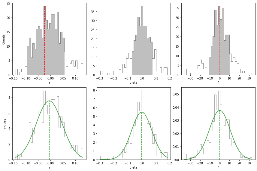
Again, if you wish to write the result (to avoid having to run the previous box again), just set write=True. This will pickle the result:
[45]:
write=False

if write:
    output = {'speckle_res':speckle_res}
    with open('../datasets/my_speckle_residuals_results', 'wb') as fileSave:
        pickle.dump(output, fileSave)
Load pickled results from disk:
[46]:
with open('../datasets/speckle_residuals_results','rb') as fi:
    myPickler = pickle.Unpickler(fi)
    sp_unc_result = myPickler.load()

print(sp_unc_result.keys())

speckle_res = sp_unc_result['speckle_res']
sp_unc, mean_dev, p_simplex, offset, chi2, nit, success = speckle_res
dict_keys(['speckle_res'])
The speckle uncertainty associated to each parameter is contained in sp_unc which corresponds to the 1\(\sigma\) width of a Gaussian distribution fitted to the offset distribution (i.e. the differences with respect to injected ground truths):
[47]:
sp_unc
[47]:
array([ 0.05350939, 0.07376633, 10.64773837])
For comparison, the uncertainties found by the MCMC procedure were:
[48]:
sigma
[48]:
array([ 0.13676103, 0.15744912, 21.66963444])
5.3.5. Final uncertainties
The final uncertainties on the planet parameters should include both statistical and systematic uncertainties. The former include both the photon noise and residual speckle noise uncertainties discussed above. The latter include both the uncertainty on the star location (which may be non-negligible when using a coronagraph) and instrumental calibration errors, including:
- the uncertainty on the plate scale (for \(r\), when converting to angular separation) - note that it is proportional to the radial separation itself;
- the uncertainty on the PA of true north (for \(\theta\)).
The uncertainty on the star location is of the order of 0.3px in individual NACO+AGPM images (this is the typical precision by manual recentering during the observation). Given the shift plots in Tutorial 2, it appears the autocorrelation timescale is of the order of ~5 frames. Therefore, considering that there are 61 frames in the datacube, the uncertainty on the star location in the final combined image must be roughly:
[49]:
cen_unc_indiv = 0.3 #px
cen_unc = cen_unc_indiv/np.sqrt(61/5) #px
cen_unc
[49]:
0.08588975014708022
The latter can be translated into an uncertainty on \(\theta\) by division by the radial separation of the companion. The stellar centering uncertainties on each planet parameter can thus be expressed as:
[50]:
star_unc = np.array([cen_unc*pxscale_naco,
                     np.rad2deg(cen_unc/val_max['r']),
                     0]) # uncertainty on each of the 3 parameters due to stellar centering
where the multiplication by pxscale_naco has converted the radial separation in arcsec.
For the instrumental calibration errors, we adopt the values quoted in Absil et al. (2013). Note that the uncertainty related to the plate scale is directly proportional to the radial separation of the companion.
[51]:
dr_unc = 0.00004 # plate scale uncertainty in arcsec per px
tn_unc = 0.09    # deg
syst_unc = np.array([val_max['r']*dr_unc,
                     tn_unc,
                     0])
The final uncertainties are then the different sources of uncertainty added quadratically - after conversion of the radial separation to arcsec:
[52]:
sigma[0] *= pxscale_naco
sp_unc[0] *= pxscale_naco

if mu_sigma:
    final_unc = np.sqrt(np.power(sigma,2) + np.power(star_unc,2) + np.power(syst_unc,2))
else:
    final_unc = np.sqrt(np.power(sigma,2) + np.power(sp_unc,2) + np.power(star_unc,2) + np.power(syst_unc,2))
[53]:
msg = "The final estimates on the radial separation, PA and flux of the companion, including uncertainties, are: \n"
msg+= "r = {:.2f}+-{:.2f} mas (GT: {:.2f} mas), \n"
msg+= "PA = {:.2f}+-{:.2f} deg (GT: {:.2f} deg) \n"
msg+= "f = {:.2f}+-{:.2f} ADUs (GT: {:.2f} ADUs)"
print(msg.format(val_max['r']*pxscale_naco*1000, final_unc[0]*1000, rad_fc*pxscale_naco*1000,
                 val_max['theta'], final_unc[1], theta_fc,
                 val_max['f'], final_unc[2], flux_fc))
The final estimates on the radial separation, PA and flux of the companion, including uncertainties, are:
r = 831.33+-4.56 mas (GT: 829.29 mas),
PA = 239.92+-0.24 deg (GT: 240.00 deg)
f = 390.77+-21.67 ADUs (GT: 400.00 ADUs)
Let’s consider the Gaussian fit instead:
[54]:
msg = "Considering a Gaussian fit to the posterior distributions, the final estimates on the radial separation, PA and flux of the companion, including uncertainties, are: \n"
msg+= "r = {:.2f}+-{:.2f} mas (GT: {:.2f} mas), \n"
msg+= "PA = {:.2f}+-{:.2f} deg (GT: {:.2f} deg) \n"
msg+= "f = {:.2f}+-{:.2f} ADUs (GT: {:.2f} ADUs)"
print(msg.format(mu[0]*pxscale_naco*1000, final_unc[0]*1000, rad_fc*pxscale_naco*1000,
                 mu[1], final_unc[1], theta_fc,
                 mu[2], final_unc[2], flux_fc))
Considering a Gaussian fit to the posterior distributions, the final estimates on the radial separation, PA and flux of the companion, including uncertainties, are:
r = 830.00+-4.56 mas (GT: 829.29 mas),
PA = 239.95+-0.24 deg (GT: 240.00 deg)
f = 394.13+-21.67 ADUs (GT: 400.00 ADUs)