1A. Quick-start

Authors: Valentin Christiaens and Carlos Alberto Gomez Gonzalez

Suitable for VIP v1.0.3 onwards

Last update: 2024/03/04

Table of contents

• 1.1. Loading ADI data

• 1.2. PSF subtraction

  • 1.2.1. median-ADI

  • 1.2.2. Full-frame PCA

• 1.3. Is the point source significant?

This quick-start tutorial shows:

• how to load Angular Differential Imaging (ADI) datacubes;

• how to use algorithms implemented in VIP to model and subtract the stellar halo, and search for faint circumstellar companions in the post-processed images;

• how to quickly assess the significance of a point source found in a post-processed image.

---

Let’s assume VIP is properly installed. If not, follow the instructions here. We import the package along with other useful packages which are installed together with VIP. The hciplot package aims to be the “Swiss army” solution for plotting and visualizing multi-dimensional high-contrast imaging datacubes.

import vip_hci as vip

from hciplot import plot_frames, plot_cubes
from matplotlib import pyplot as plt
import numpy as np

In the following box we check that your version of VIP is recent enough to run this notebook. It should be >=1.0.3. If not, close the notebook and run for example pip install vip_hci --upgrade in your terminal.

from packaging import version
vvip = vip.__version__
print("VIP version: ", vvip)
if version.parse(vvip) < version.parse("1.0.3"):
    msg = "Please upgrade your version of VIP"
    msg+= "It should be 1.0.3 or above to run this notebook."
    raise ValueError(msg)

VIP version:  1.6.0

VIP also allows interactive work with DS9 provided that it’s installed on your system along with pyds9. A DS9 session (window) can be started with:

ds9 = vip.Ds9Window()

If the above fails but you have pyds9 installed (vip_ds9 is only a wrapper around pyds9), you may find the following troubleshooting tips useful (e.g. step 4).

The ds9 methods will allow interaction with the DS9 window. For example, for sending an array to the DS9 window you can simply use:

ds9.display(2d_or_3d_array)

The above can be used instead of hciplot’s plot_frames and plot_cubes routines (the latter being used in this notebook) for visualization and interaction with your images/datacubes.

1.1. Loading ADI data

In order to demonstrate the capabilities of VIP, you can find in the ‘dataset’ folder of the VIP_extras repository: - a toy Angular Differential Imaging (ADI) datacube of images (naco_betapic_cube_cen.fits), - the associated parallactic angles, indicating the direction of true north in each image of the datacube (naco_betapic_pa.fits), - a non-coronagraphic point spread function (naco_betapic_psf.fits).

The dataset was obtained with the NACO instrument of the Very Large Telescope (VLT). This is an L’-band dataset of beta Pictoris published in Absil et al. (2013), obtained using the Annular Groove Phase Mask (AGPM) Vortex coronagraph. The sequence has been heavily sub-sampled temporarily to make it smaller. The frames were also cropped to the central 101x101 area. In case you want to plug-in your cube just change the path of the following cells.

Let’s load a couple of utilities related to fits files:

from vip_hci.fits import open_fits, write_fits, info_fits

Let’s first inspect the fits file using the info_fits function:

info_fits('../datasets/naco_betapic_cube_cen.fits')

Filename: ../datasets/naco_betapic_cube_cen.fits
No.    Name      Ver    Type      Cards   Dimensions   Format
  0  PRIMARY       1 PrimaryHDU       7   (101, 101, 61)   float32

The fits file contains an ADI datacube of 61 images 101x101 px across. The length of the parallactic angle vector for this observation is thus also 61.

Now let’s load all the data in memory with the open_fits function:

psfname = '../datasets/naco_betapic_psf.fits'
cubename = '../datasets/naco_betapic_cube_cen.fits'
angname = '../datasets/naco_betapic_pa.fits'

cube = open_fits(cubename)
psf = open_fits(psfname)
angs = open_fits(angname)

FITS HDU-0 data successfully loaded. Data shape: (61, 101, 101)
FITS HDU-0 data successfully loaded. Data shape: (39, 39)
FITS HDU-0 data successfully loaded. Data shape: (61,)

As a reminder, you can use ‘?’ after a given function to know what it requires as input, and what it returns as output. For example:

open_fits?

Signature:
open_fits(
    fitsfilename,
    n=0,
    header=False,
    ignore_missing_end=False,
    precision=<class 'numpy.float32'>,
    return_memmap=False,
    verbose=True,
    **kwargs,
)
Docstring:
Load a fits file into memory as numpy array.

Parameters
----------
fitsfilename : string or pathlib.Path
    Name of the fits file or ``pathlib.Path`` object
n : int, optional
    It chooses which HDU to open. Default is the first one. If n is equal
    to -2, opens and returns all extensions.
header : bool, optional
    Whether to return the header along with the data or not.
precision : numpy dtype, optional
    Float precision, by default np.float32 or single precision float.
ignore_missing_end : bool optional
    Allows to open fits files with a header missing END card.
return_memmap : bool, optional
    If True, the function returns the handle to the FITS file opened by
    mmap. With the hdulist, array data of each HDU to be accessed with mmap,
    rather than being read into memory all at once. This is particularly
    useful for working with very large arrays that cannot fit entirely into
    physical memory.
verbose : bool, optional
    If True prints message of completion.
**kwargs: optional
    Optional arguments to the astropy.io.fits.open() function. E.g.
    "output_verify" can be set to ignore, in case of non-standard header.

Returns
-------
hdulist : HDU or HDUList
    [memmap=True] FITS file ``n`` hdulist. If n equals -2, returns the whole
    hdulist.
data : numpy ndarray or list of numpy ndarrays
    [memmap=False] Array containing the frames of the fits-cube. If n
    equals -2, returns a list of all arrays.
header : dict or list of dict
    [memmap=False, header=True] Dictionary containing the fits header.
    If n equals -2, returns a list of all dictionaries.
File:      ~/GitHub/VIP/vip_hci/fits/fits.py
Type:      function

open_fits is a wrapper of the astropy fits functionality. The fits file is now a ndarray or numpy array in memory.

If you open the datacube with ds9 (or send it to the DS9 window) and adjust the cuts you will see the beta Pic b planet moving on a circular trajectory, among similarly bright quasi-static speckle. Alternatively, you can use hciplot.plot_cubes:

%matplotlib inline
plot_cubes(cube, vmin=0, vmax=400)

:Dataset   [x,y,time]   (flux)
:Cube_shape     [101, 101, 61]

Let’s fit the PSF with a 2D Gaussian to infer the FWHM, determine the flux in a 1-FWHM size aperture, and get a flux-normalized PSF. This is done in the normalized_psf function defined in the forward modeling (fm) subpackage:

%matplotlib inline
from vip_hci.fm import normalize_psf  # fm is the forward modeling subpackage, with various tools for the characterization of point sources and extended signals.

psfn, flux, fwhm_naco = normalize_psf(psf, size=19, debug=True, full_output=True)

FWHM_y = 4.926059872957138
FWHM_x = 4.675778895005929

centroid y = 9.010992107833063
centroid x = 9.01917912265807
centroid y subim = 9.010992107833063
centroid x subim = 9.01917912265807

amplitude = 0.10032285220380603
theta = -38.446187060503874

Mean FWHM: 4.801
Flux in 1xFWHM aperture: 1.307

print(fwhm_naco)

4.800919383981533

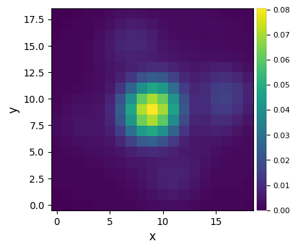
Now let’s visualize the normalized PSF with hciplot.plot_frames. Feel free to adapt the backend argument throughout the notebook: backend='matplotlib' (default) allows paper-quality figures with annotations which can be saved, while backend='bokeh' enables interactive visualization.

plot_frames(psfn, size_factor=4)#, backend='bokeh')

Let’s finally define the pixel scale for NACO (L’ band), which we get from a dictionary stored in the config subpackage:

from vip_hci.config import VLT_NACO  # config is a subpackage with configuration files and parameter/dictionary definition

pxscale_naco = VLT_NACO['plsc']
print(pxscale_naco, "arcsec/px")

0.02719 arcsec/px

1.2. PSF subtraction

When loading the ADI cube above, we assumed all calibration and preprocessing steps were already performed. In particular, the star is assumed to be already centered in the images. If your data require additional calibration/preprocessing, check out tutorial 2. Pre-processing.

IMPORTANT - VIP’s convention regarding star centering is: - for odd number of pixels along the x and y directions: the star centroid corresponds to the central pixel of the image; - for even number of pixels: the star centroid is located on coordinates (dim/2,dim/2) in 0-based indexing.

1.2.1. median-ADI

The most simple approach is to model the PSF with the median image of the ADI sequence, subtract it, then derotate and median-combine all residual images (Marois et al. 2006):

from vip_hci.psfsub import median_sub

fr_adi = median_sub(cube, angs)

――――――――――――――――――――――――――――――――――――――――――――――――――――――――――――――――――――――――――――――――
Starting time: 2024-03-04 22:28:33
――――――――――――――――――――――――――――――――――――――――――――――――――――――――――――――――――――――――――――――――
Median psf reference subtracted
Done derotating and combining
Running time:  0:00:02.032495
――――――――――――――――――――――――――――――――――――――――――――――――――――――――――――――――――――――――――――――――

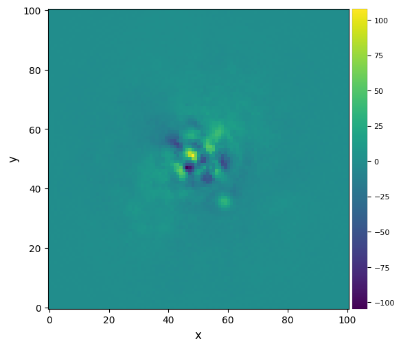
Let’s visualize the final images:

plot_frames(fr_adi)

Strong residuals can be seen near the center of the image, with a faint potential point source in the south-west (bottom right) of the final image.

1.2.2. Full-frame PCA

Now let’s try the Principal Component Analysis (PCA) algorithm (Amara & Quanz 2012, Soummer et al. 2012), and set to 5 the number of principal components ncomp considered to create the model PSF.

from vip_hci.psfsub import pca    # psfsub is the subpackage containing PSF modeling and subtraction algorithms

fr_pca1 = pca(cube, angs, ncomp=5)

――――――――――――――――――――――――――――――――――――――――――――――――――――――――――――――――――――――――――――――――
Starting time: 2024-03-04 22:28:35
――――――――――――――――――――――――――――――――――――――――――――――――――――――――――――――――――――――――――――――――
System total memory = 17.180 GB
System available memory = 3.894 GB
Done vectorizing the frames. Matrix shape: (61, 10201)
Done SVD/PCA with numpy SVD (LAPACK)
Running time:  0:00:00.051901
――――――――――――――――――――――――――――――――――――――――――――――――――――――――――――――――――――――――――――――――
Done de-rotating and combining
Running time:  0:00:02.235239
――――――――――――――――――――――――――――――――――――――――――――――――――――――――――――――――――――――――――――――――

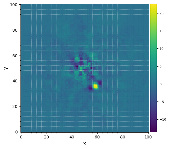
Let’s visualize the final image. This time let’s set the grid option on, to better read coordinates from the image. Alternatively, use the backend='bokeh' option for interactive reading:

plot_frames(fr_pca1, grid=True)#, backend='bokeh')

The improvement is clear compared to previous reductions. Very low residuals are seen near the star, and the companion candidate appears as a bright point source surrounded by negative side-lobes.

1.3. Is it significant?

Now let’s see whether the candidate is significant. For that let’s first set the x,y coordinates of the test point source based on the above image:

xy_b = (58.5,35.5)

Let’s compute the signal-to-noise ratio at that location, following the definition in Mawet et al. (2014), using the appropriate function defined in the metrics subpackage:

from vip_hci.metrics import snr

snr1 = snr(fr_pca1, source_xy=xy_b, fwhm=fwhm_naco)
print(r"S/N = {:.1f}".format(snr1))

S/N = 7.7

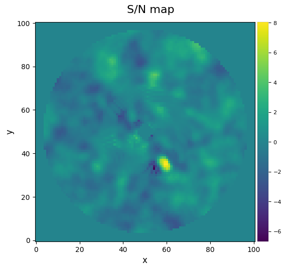
One can also calculate a S/N ratio map over the whole image (this may take a couple of seconds depending on the size of your image):

from vip_hci.metrics import snrmap

snrmap1 = snrmap(fr_pca1, fwhm_naco, plot=True)

――――――――――――――――――――――――――――――――――――――――――――――――――――――――――――――――――――――――――――――――
Starting time: 2024-03-04 22:28:37
――――――――――――――――――――――――――――――――――――――――――――――――――――――――――――――――――――――――――――――――

S/N map created using 5 processes
Running time:  0:00:02.474484
――――――――――――――――――――――――――――――――――――――――――――――――――――――――――――――――――――――――――――――――

Remember that S/N ratio is NOT the same as significance (Mawet et al. 2014). Let’s convert the measured S/N ratio (Students statistics) into a Gaussian “sigma” with equivalent false alarm probability. This first involves calculating the radial separation of the candidate, for which we use the frame_center and dist convenience routines to infer the pixel coordinates of the center, and the radial separation of the point source, respectively:

from vip_hci.var import frame_center, dist   # var is a subpackage containing various utility routines

cy, cx = frame_center(snrmap1)
rad = dist(cy, cx, xy_b[1], xy_b[0])

Now let’s use the significance routine in VIP to operate the conversion:

from vip_hci.metrics import significance

sig = significance(snr1, rad, fwhm_naco, student_to_gauss=True)

At a separation of 16.8 px (3.5 FWHM), S/N = 7.7 corresponds to a 5.2-sigma detection in terms of Gaussian false alarm probability.

Congratulations! The detection is significant! You obtained a conspicuous direct image of an exoplanet! Although from this image alone (at a single wavelength) one cannot disentangle a true physically bound companion from a background star, this source has now been extensively studied: it corresponds to the giant planet beta Pic b (e.g. Lagrange et al. 2009, Absil et al. 2013).

You’re now ready for more advanced tutorials. If you wish to know more about:

• basic usage but using an object-oriented framework –> go to Tutorial 1B;

• pre-processing functionalities available in VIP (star centering, bad frame trimming, bad pixel correction…) –> go to Tutorial 2;

• more advanced post-processing algorithms –> go to Tutorial 3A or 3B (the latter for Object-Oriented example usage);

• metrics to evaluate the significance of a detection or the achieved contrast in your image –> go to Tutorial 4;

• how to characterize a directly imaged companion –> go to Tutorial 5A;

• how to characterize a circumstellar disk –> go to Tutorial 5B;

• how to characterize a companion in a disk using JWST observations –> go to Tutorial 5C (to come soon);

• post-processing algorithms leveraging reference star differential imaging –> go to Tutorial 6 (to come soon);

• post-processing algorithms leveraging spectral differential imaging –> go to Tutorial 7;

• the difference between FFT- and interpolation-based image operations (rotation, shifts, scaling) –> go to Tutorial 8;